Project 5 - Diffusion Tensor Visualization

Key Dates
Handed out: November 11, 2015
Due: Friday, November 27, 2015 before 8:00 am
Objective
The topic of this final assignment is tensor field visualization. Specifically, you will study a medical dataset obtained by diffusion weighted tensor imaging of a healthy human brain. Your task consists in applying glyphs, so-called hyperstreamlines, and volume rendering to reveal the geometric structure of the white matter present in this dataset.
Tasks
Task 1: Glyphs
Similar to what you did in the fifth assignment, your first task consists in combining cutting planes and glyphs to visualize the tensor values contained in the DTI dataset. Specifically, you will select 3 planes corresponding to sagittal, coronal, and transverse views of the data. On each plane, you will sample the corresponding tensor values and display them with the help of vtkTensorGlyph. More precisely, I am asking you to create ellipsoid glyphs and to color code them according to the orientation of the major eigenvector. Refer to the examples provided here. Note that you need to use the modified version of vtkTensorGlyph provided at the bottom of this page to achieve the requested color mapping since it is not supported by the original VTK implementation.
Note: You will be using ellipsoid glyphs despite the limitations that we have discussed in class because superquadric glyphing is vtkSuperQuadricTensorGlyphFilter.
Deliverables: Create an executable named tensor_glyphs[.py] that contains the (hardcoded) information needed to create the requested visualization. Your executable should receive the name of the DTI data file from the command line.
> tensor_glyphs <dti.vtk>
Report: Include in your report pictures showing each cutting plane individually (along with the associated glyphs) as well as other images showing all planes together.
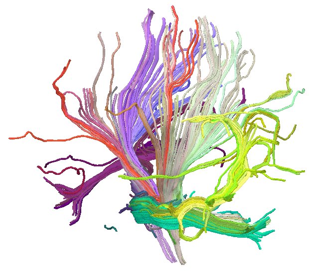
Task 2: Hyperstreamlines
Using the information gathered in Task 1 about the location of of major anatomical structures of the white matter, your second task now consists in using vtkHyperStreamline. Here, hyperstreamlines will capture fiber tracts in the DTI dataset. Note that hyperstreamlines (with their elliptical cross section scaling) are not ideally suited to represent fiber tracts. That is why I am providing you with a slightly modified version of this class that will allow you to turn off the elliptical tube wrapping to simply produce a curve tangential to the major eigenvector field in the case of the DTI dataset. Practically, you will select a number of seed points (between 10 and 50) on each plane chosen in Task 1 and integrate hyperstreamlines in both directions from each seed. Again, you will need to use the modified vtkHyperstreamline implementation provided at the bottom of the page.
Deliverables: Create an executable named hyperstreamlines that contains hardcoded parameters to generate all the hyperstreamlines that you have selected. As always, the input DTI file will be passed to your program on the command line.
> hyperstreamlines <dti.vtk>
Report: Describe in the report how the seeding locations were selected and comment on the quality of the results that you were able to produce with this method.
Task 3: Volume Rendering and Fibers
An alternative way to analyze tensor fields consists in visualizing some properly selected scalar invariants using scalar field visualization techniques. In the context of diffusion tensor imaging, a popular invariant is fractional anisotropy (FA), which measures the degree to which the local diffusion tensor corresponds to a purely anisotropic diffusion in a single direction. Specifically, FA is derived from the eigenvalues according to following formula. $$\mbox{FA}\, = \,\sqrt{\frac{3}{2}}\, {\left|\mathbf{\Lambda}\,-\,\overline{\lambda}\mathbf{I}\right|}\,/\,{\left|\mathbf{\Lambda}\right|},$$ with $\mathbf{\Lambda}\, := \, \left(\lambda_1, \lambda_2, \lambda_3\right)^T$ is the column vector representation of the three eigenvalues of the diffusion tensor, $\left|\cdot\right|$ is the vector norm, $\overline{\lambda}\, := \, \frac{1}{3}\left(\lambda_1 + \lambda_2 + \lambda_3\right)$ is the average of all three eigenvalues, and $\mathbf{I} = \left( 1, 1, 1 \right)^T$.
For this third task, I am asking you to visualize through volume rendering the FA field provided in a separate file together with the hyperstreamlines that you constructed in Task 2. To design a suitable transfer function for FA, you should use the code that you wrote for this purpose in Project 3 to determine the control points of your opacity transfer function. Your color transfer function should be uniformly white.
Deliverables: Create and executable named fa_hyper[.py] that visualizes the DTI dataset through the requested combination of volume rendering of FA and fiber tracts of the diffusion tensor field. The settings of hyperstreamlines / fiber tracts must be hardcoded in your program. Similarly, the opacity transfer function must be defined explicitly in your code. Your executable will receive from the command line the names of the DTI file on one hand and of the FA dataset on the other hand.
> fa_hyper <dti.vtk> <fa.vtk>
Report: Describe in the report the procedure you followed to select your transfer function. Compare the results that you obtained with this method to those obtained with the hyperstreamlines alone in Task 2.
Data Sets
The data available for this project consists of a diffusion tensor MRI dataset and of the corresponding fractional anisotropy scalar dataset. This medical dataset was part of the IEEE Visualization Challenge 2010 and is courtesy of Prof. B. Terwey, Klinikum Mitte, Bremen, Germany. As mentioned previously, the data is comprised of two files: one corresponding to the diffusion tensor information and one corresponding to the fractional anisotropy. The data has been cleaned and diffusion tensor values outside of the white matter have been uniformly set to zero. Both files are of type vtkStructuredPoints with float precision. The FA dataset is also provided in unsigned short precision to facilitate its volume rendering with VTK. The resolution of the voxel grid is 128 x 128 x 72.
- Diffusion Tensor MRI dataset (tensor field,
floatprecision): dti.vtk (41 MB) - Fractional Anisotropy (scalar field): fa.vtk (
float, 4.5 MB) / fa_short.vtk (unsigned short, 2.3 MB)
Modified VTK Code
As stated previously, the versions of vtkTensorGlyph and vtkHyperStreamline implemented in the current release of VTK do not support the type of visualizations that I ask you to create for this assignment. I am therefore providing you with modified implementations that address these shortcomings. To use these files in your code, you will need to copy them in the VTK source tree and recompile VTK. Fortunately, this should only require the recompilation of a small portion of the overall VTK source code.
vtkTensorGlyph.handvtkTensorGlyph.cxx(to be copied underVTK/Filters/Core). Use the methodSetColorModeToEigenvector()to achieve the requested directional color coding.vtkHyperStreamline.handvtkHyperStreamline.cxx(to be copied underVTK/Filters/General). Use the methodTubeWrappingOff()to create a line in output instead of a tube.
Submission
Submit your solution for this project before Friday, November 27, 2015 before 8:00 am . Refer to the instructions below.
- Include all program files (
tensor_glyphs,hyperstreamlines,fa_hyper) along with any other source code you may have. - Include
Makefile(resp.CMakeLists.txt) (if applicable). If you are using Visual Studio include the solution file (.sln) and the project files (.vcproj) that are needed to build your project. - Include high resolution sample images showing results for each task.
- Include a html or PDF report summarizing what you have done and answering all the questions asked. The report should include high-resolution images.
- Include
README.txtfile with compilation / execution instructions (optional). - Include all submitted files in a single directory named
<myLogin>_p5, where<myLogin>is your Purdue login. - Do not include binary file
- Do not include data files
- Do not use absolute paths in your code
After logging into
data.cs.purdue.edu, submit your assignment as
follows:
> turnin -c cs530 -p project5
          <dir_name>
where <dir_name> is the name
of the directory containing all your submission material for Project 5.
Keep in mind that old submissions are overwritten by new ones whenever you execute this command. You can verify the contents of your submission by executing the following command:
> turnin -v -c cs530 -p
          project5
Do not forget the -v flag here, as
otherwise your submission would be replaced by an empty one.