CS530 - Spring 2018
Project 4 - Vector Field Visualization

Stream surface
visualization of a vortex breakdown bubble Finite-time Lyapunov exponent of a turbulent
flow

Key Dates

Handed out: March 12, 2018

Due: April 2, 2018 before 11:59 pm

Objective

The topic of this assignment is vector field / flow visualization. You will study a delta wing dataset similar to the one you visualized in the second part of project 3. This time, you will visualize the velocity information using vector field visualization techniques. Your objective will be to show the major flow structures present in the dataset (primary and secondary vortices and recirculation bubble on each side of the wing).

The second part of this assignment is an optional Part 2 that counts toward extra credit. The topic of the second part is tensor field visualization. Your task consists in applying glyphs, so-called hyperstreamlines, and volume rendering to reveal the geometric structure of a stress tensor field dataset.

Part 1 [100%]

Task 1: Glyphs [20%]

Your first task consists in using a cutting plane to probe the vector values. Specifically, I am asking you to create a plane orthogonal to the X axis of the volume and to sample the velocity vector field on that plane. You will need to follow an approach similar to what is demonstrated in Graphics/Testing/Tcl/probe.tcl for that purpose. To represent individual vectors as arrows, you will use vtkArrowSource and use it as the source of a vtkGlyph3D filter. Use 3 plane at 3 different locations along the X axis (with normal pointing along the X direction) to capture the structures mentioned above. Show the delta wing geometry in each image for context (the corresponding geometry is provided as vtkUnstructuredGrid in a separate file).

Deliverables: Create an executable named three_planes[.py] that contains the (hardcoded) information needed to visualize the vector glyphs on the 3 planes that you have selected. Your executable should receive the names of two files from the command line, namely the CFD file containing the vector field information and the file containing the geometry of the delta wing.

> three_planes <tdelta.vtk> <wing.vtk>

Report: Explain in the report how you selected the planes used in your implementation and comment on the properties of the flow that you can discern in your visualization. Include pictures showing each cutting plane individually (along with the associated glyphs) as well as other images showing all planes and the wing together.

Task 2: Streamlines, Stream Tubes and Stream Surfaces [40%]

Task 1 should provide you with a general sense of the location of interesting structures in the flow volume. Your second task now consists in using streamlines, stream tubes and stream surfaces as demonstrated in Examples/VisualizationAlgorithms/Python/officeTube.py and Examples/VisualizationAlgorithms/Python/streamSurface.py to show how the flow swirls around the vortices present in the data.

Deliverables: You will construct 3 visualizations for this task.

A first executable showing a large number (at least 50) of streamlines.
A second executable showing a small number of stream tubes
A third executable showing a stream surface seeded along an appropriately chosen rake.

In each case, the seeding locations and the other parameters of the technique must be hardcoded in your program. You must choose parameter values that produce good quality results and capture the behavior of the flow around the vortices on each side of the wing. Note that each visualization should represent the velocity magnitude using color coding and the corresponding color scale should be provided for reference. Show the delta wing geometry in each image for context.

> streamlines <tdelta.vtk> <wing.vtk>
> streamtubes <tdelta.vtk> <wing.vtk>
> streamsurfaces <tdelta.vtk> <wing.vtk>

Report: Explain in the report how the seeding locations were chosen for each of these three techniques and how they relate to the observations made in Task 1.

Task 3: Combining Scalar and Vector Visualization [20%]

The scalar and vector information available for this dataset provide two complementary perspectives on the properties of the flow. For the third task of this assignment, you will combine isosurfaces of vorticity magnitude with streamlines to visualize the relationship between the streamlines’ geometry and the shape of the isosurfaces. Create visualizations in which the streamline seeds and the isovalues of the isosurface are chosen in such a way as to best illustrate the correlation between the two kinds of object.

Deliverables: Create and executable named combined[.py] that produces a visualization of the CFD dataset, combining isosurfaces of the vorticity magnitude, streamlines of the velocity vector field, and geometry of the delta wing. The various parameters needed to create the visualization must be hardcoded in the program. Your executable should receive from the command line the names of the three files needed to create the visualization: velocity dataset, vorticity dataset, and wing geometry description.

> combined <tdelta.vtk> <vorticity.vtk> <wing.vtk>

Report: Describe in the report the things you tried before arriving at the proposed solution and explain why your final selection is a good one. Show the delta wing geometry in each image for context.

Task 4: Analysis [20%]

Considering your results in Task 1 and Task 2 of the assignment, comment on the effectiveness of the resulting visualizations for your understanding of this dataset. What were the pros and cons of each technique? Comment on the results you were able to achieve in Task 3 by integrating isosurfacing and vector visualization. Did you find this combination beneficial? Provide a justified answer to each of these questions in the report.

Part 2: Tensor Visualization (Extra credit) [50%]

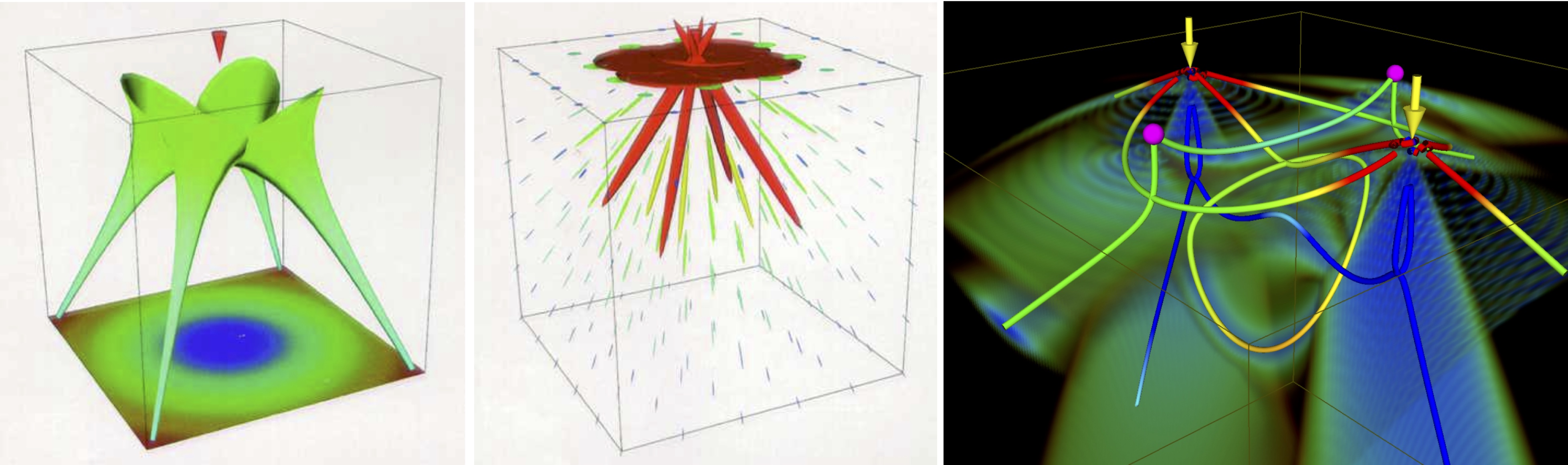
Overview

The purpose of this second (and optional) part of Project 4 is to visually inspect a stress tensor field using standard tensor visualization techniques. The dataset that you will use corresponds to the superimposition of two point loads. This dataset has been widely used in the tensor visualization literature (see e.g., the reference hereafter) and it offers a good experimentation basis for this project.

Task 1: Glyphs

Similar to what you did in Part 1, your first task consists in combining cutting planes and glyphs to visualize individual values of the stress tensor dataset. Here, you will select 3 to 5 planes orthogonal to the X, Y, or Z axes, and on each plane you will sample the corresponding tensor values and display them with the help of vtkTensorGlyph. More precisely, I am asking you to create ellipsoid glyphs and to color code them according to the trace of the stress tensor. Refer to the examples provided here.

Note: You will be using ellipsoid glyphs despite the limitations that we will discuss in class because superquadric glyphing is not available in the current release of VTK (8.2).

Deliverables: Create an executable named tensor_glyphs[.py] that contains the (hardcoded) information needed to create the requested visualization. Your executable should receive the name of the tensor data file from the command line.

> tensor_glyphs <dpl.vtk>

Report: Include in your report pictures showing each cutting plane individually (along with the associated glyphs) as well as other images showing all planes together. Pay attention to the scaling factor of the tensor glyphs in order to create images in which the glyphs are clearly visible, yet do not occlude each other too much. You will find the clamping mechanism available for the scale factor convenient in that regard.

Task 2: Hyperstreamlines

Using the information gathered in Part 2 Task 1 about the location of interesting structures (and in particular the various symmetries) of the stress tensor field, your second task consists in using vtkHyperStreamline. You will apply hyperstreamlines to both the major and the minor eigenvector field of the stress tensor. Practically, you will select for each eigenvector field a number of seed points (between 5 and 20, e.g., on the plane chosen in Part 2 Task 1) and integrate hyperstreamlines from each seed.

Deliverables: Create an executable named hyperstreamlines that contains hardcoded parameters to generate all the hyperstreamlines that you have selected. As always, the input dataset will be passed to your program on the command line.

> hyperstreamlines <stress.vtk>

Report: Describe in the report how the seeding locations were selected and comment on the quality of the results that you were able to produce with this method. In particular, compare the respective benefits of glyphs and hyperstreamline to analyze this dataset.

Data Sets

Part 1

As stated above, the CFD dataset used in this project is very similar to the one you visualized in the previous assignment. The data is available in high and low resolution versions. In each case, the information available corresponds to the velocity (vector field) and the vorticity magnitude (a scalar field). A file describing the geometry of the delta wing is also available that will provide a geometric context to your visualizations. Note that while the CFD simulation that produced this dataset was computed over an unstructured grid, all the datasets included in this project are of type vtkStructuredPoints with float precision, at the exception of the wing (vtkUnstructuredGrid).

Velocity (vector field, float precision): low resolution (69 MB) / high resolution (549 MB)
Vorticity magnitude (scalar field, float precision): low resolution (23 MB) / high resolution (183 MB)
Wing geometry (mesh only, 7 MB )

Part 2

The data available for the second part of this project consists of a stress tensor obtained procedurally through the combination of two point loads applied on a semi-infinite solid. The corresponding formulae are borrowed from vtkPoinLoad. The data is of type vtkStructuredPoints. The tensor field is given in float precision and available in low and high resolutions.

Stress tensor field (tensor field, float precision): low resolution dpl-small.vtk (1.8 MB) and high resolution dpl-large.vtk (14 MB)

Submission

Submit your solution for this project before April 02, 2018 at 11:59 pm.

Include all source code you have.
Include Makefile (resp. CMakeLists.txt) (if applicable). If you are using Visual Studio include the solution file (.sln) and the project files (.vcproj) that are needed to build your project.
If you are submitting python code, please add "#! python2" at the beginning of the file, if you are using Python 2.7, and add "#! python3" if you are using python 3.x. This is to make my grading life easier. (See here for detail on py launcher)
Include high resolution sample images showing results for each task.
Include a PDF report briefly summarizing what you have done and answering all the questions asked. As always, the report should include high-resolution images.
Include README.txt file with compilation / execution instructions (optional).
Include all submitted files in a single directory named <myLogin>_p4, where <myLogin> is your Purdue login.
Do not include binary file
Do not include data files
Do not use absolute paths in your code

Put all your files in a folder and package your folder to a zip file. Submit your file through Blackboard submit. You can do so by logging into Blackboard, go to Course Content on the left column, and click on the "Assignment: Project 4" link. There will be a section to attach files. Please make sure your file size is less than 20MB. Do not leave your submission to last minute, as often time Blackboard would be overloaded with requests and hang, and you may not get your submission uploaded on-time.