Project 5: Vector Field / Flow Visualization
Handed out: Tuesday, April 13, 2013
Due: Tuesday, April 28, 2013
Purpose
As expected, the topic of this fifth (and last!) assignment is vector field / flow visualization. In contrast to previous projects, this project is in fact two projects in one.
The first part corresponds to the study of a delta wing dataset similar to the one you visualized in project 4. This time however you will be visualizing the velocity information using the vector field visualization techniques supported by VTK. Your objective in this part will be to capture with your visualization the major flow structures present in the dataset (primary and secondary vortices and recirculation bubble on each side of the wing).
The second part of the project is concerned with the implementation of a high quality stream surface computation algorithm. The basic idea of the solution you will consider is to use the correspondence between the geometry of the stream surface and its canonical 2D parameterization (see explanations below). This part is meant for students who feel comfortable tackling a moderately complicated coding task within a limited time frame. Once implemented, you will apply your stream surface algorithm to the delta wing dataset to showcase your technique.
Note that each part amounts to full credit for this project so you can choose which part to complete.
Part 1 - Visual Exploration of a Delta Wing Dataset [100%]
Task 1 : Glyphs [20%]
Your first task consists in using a cutting plane to probe the vector values. Specifically, I am asking you to create a plane orthogonal to the X axis of the volume and to sample the velocity field on that plane. You will need to follow an approach similar to what is demonstrated in Graphics/Testing/Tcl/probe.tcl for that purpose. To represent individual vectors as arrows, you will use vtkArrowSource and use it as the source of a vtkGlyph3D filter. Use 3 plane at 3 different locations along the X axis (with normal pointing along the X direction) to capture the structures mentioned above (explain in the report how the locations were chosen and what observations led to your decision). Show the delta wing geometry in each image for context (the corresponding geometry is provided as vtkUnstructuredGrid in a separate file). (threeplanes[.py])
> threeplanes[.py] <filename>
Task 2: Streamlines, Stream Tubes and Stream Surfaces [40%]
Task 1 should provide you with a general sense of the location of interesting structures in the volume. Now I am asking you to use streamlines, stream tubes and stream surfaces as demonstrated in Examples/VisualizationAlgorithms/*/officeTube.* and Examples/VisualizationAlgorithms/*/streamSurface.* to show how the flow swirls around the vortices present in the data. You will in fact construct 3 visualizations for this task:
-
• The first one shows a large number of streamlines (e.g., 50 or 100) (streamlines[.py])
-
• The second one shows a small number of stream tubes (streamtubes[.py])
-
• The third one shows a stream surface seeded along an appropriately chosen rake (streamsurface[.py])
In each case, the seeding locations and the other parameters of the technique should be hardcoded in your program. You must choose parameter values that produce good quality results and capture the behavior of the flow around the vortices on each side of the wing. Explain in the report how the seeding locations where chosen and how they relate to the observations made in Task 1. Note that each visualization should represent the velocity magnitude using color coding and the corresponding color scale should be provided for reference. Show the delta wing geometry in each image for context
> streamlines[.py] <filename>
> streamtubes[.py] <filename>
> streamsurface[.py] <filename>
Task 3: Combination of Scalar and Vector Visualization
The scalar and vector information available for this dataset provide two complementary perspectives on the properties of this particular flow configuration. For the third task of this assignment, I am asking you to combine isosurfaces of vorticity magnitude with streamlines to visualize the relationship between the streamlines’ geometry and the shape of the isosurfaces. Create high-quality visualizations in which the streamline seeds and the isovalues of the isosurface are chosen in such a way as to best illustrate the correlation between the two kinds of object. Be creative! (describe in the report the things you tried before arriving at the proposed solution and explain why your final selection is a good one). Show the delta wing geometry in each image for context. (combined[.py])
> combined[.py] <filename>
Task 4: Analysis [20%]
Considering your results in Task 1 and Task 2 of the assignment, comment on the effectiveness of the resulting visualizations. What were the pros and cons of each technique? Comment on the results you were able to achieve in Task 3 by integrating isosurfacing and vector visualization. Was that useful? Why? Provide a justified answer to each of these questions in the report.
Part 2 - High-Quality Stream Surface Computation [100%]
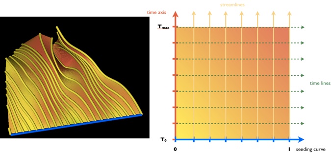
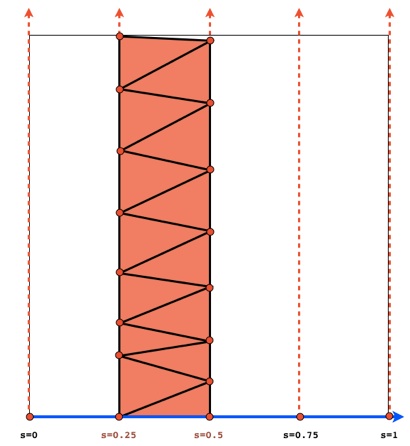
We saw in class that stream surfaces possess a natural two-dimensional parameterization whereby one dimension corresponds to the parameterization of the initial (seeding) curve and the other dimension corresponds to the integration time. These concepts are illustrated below. The left image shows a stream surface (seed curve in blue), the right image shows its corresponding 2D parameterization (seed curve parameterization from 0 to 1, time axis parameterization from T0 to Tmax).
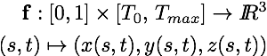
Your task in Part 2 of this project is to design and implement an algorithm that leverages the correspondence between 2D parameterization and surface in 3D to progressively refine an initially coarse stream surface until a high-quality approximation is achieved. In this framework, the stream surface is a function of two variables that associates every position in the parameter domain with the corresponding 3D position on the stream surface:
Each streamline integrated from the seed curve provides a set of points of constant s coordinate, where s is the parameter with the start location of the streamline on the seed curve. The solution that VTK implements to create a stream surface from those points consists in triangulating the space separating consecutive streamlines (i.e., creating ribbons).
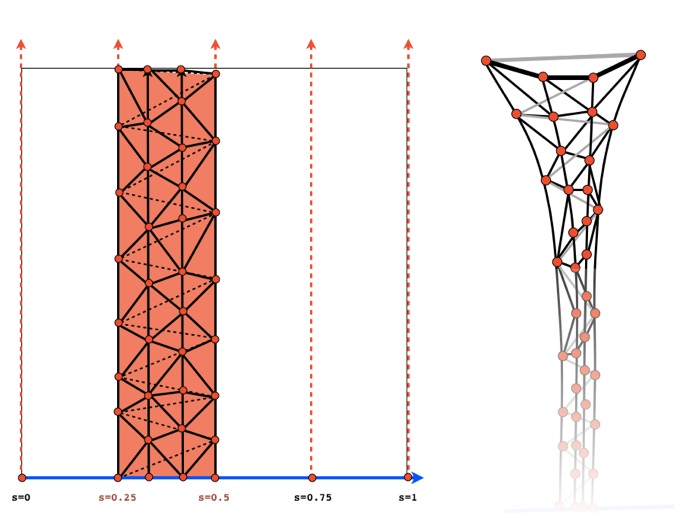
The problem with this strategy as we saw in class is that the proximity of points in the parameter domain does by no means guarantee that their associated 3D coordinates are close as well. Connecting them with triangles amounts to interpolating the space between them linearly, which is a poor approximation of the actual shape of the stream surface if it is curved. If neighboring streamlines drift away from each other, additional points are needed in the space that separates them to improve the quality of the stream surface approximation through triangles. This situation is illustrated below where the triangulation shown previously has been refined through the insertion of two additional streamlines between existing streamlines (gray edges correspond to the coarse triangulation while black edges are part of the finer triangulation).
Similarly, additional points are needed if neighboring triangles form a sharp angle along their common edge. See below.
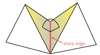
In both cases, the addition of new points to the triangulation of the parameter space requires the computation of additional streamlines from the seed curve. In summary, the successful implementation of this method requires that you come up with a way to monitor the size in 3D of the triangles that connect your points in parameter space as well as the angles that these triangles form along their edges. If these quantities exceed pre-defined thresholds (that you will need to experiment with), your algorithm should then add streamlines starting from your seed curve and re-triangulate the portion of the parameter space crossed by those new streamlines (see red region in the illustration above). Note that the triangulation in parameter space can be carried out using either a ribbon approach (see vtkRuledSurfaceFilter) or a more general 2D Delaunay strategy (see vtkDelaunay2D). Either way, the triangulation problem is a 2D one, since the connectivity between points (see vtkCellArray) can be established in parameter space and then applied to the 3D point set.
Implement a stream surface computation technique that follows this basic idea and apply it to the delta wing velocity dataset described below. Your results should showcase the visual quality that your method can achieve. Your executable (hqstreamsurface[.py]) should support following API:
> hqstreamsurface[.py] <filename> <x0> <y0> <z0> <x1> <y1> <z1> <tmax>
where (x0,y0,z0) and (x1,y1,z1) are the coordinates of the end points of the seeding segment and tmax prescribes the length of the integration.
Relevant literature
- http://vis.lbl.gov/Publications/2012/LBNL-5776E-camp.pdf
- http://dl.acm.org/citation.cfm?id=949718
Data Description
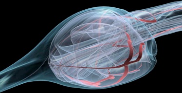
As stated above, the CFD dataset used in this project is very similar to the one you visualized in the previous assignment. The data is available in high and low resolution versions. In each case, the information available corresponds to the velocity (vector field) and the vorticity magnitude (a scalar field). I am also providing you with a dataset describing the geometry of the delta wing.
All datasets are of type vtkStructuredPoints with float precision, except for the wing (vtkUnstructuredGrid)
CFD dataset
-
-vorticity magnitude. low resolution (scalar) (float, 23 MB)
-
-velocity, low resolution (vector) (float, 69 MB)
-
-vorticity magnitude. high resolution (scalar) (float, 183 MB)
-
-velocity, high resolution (vector) (float, 549 MB)
-
-wing geometry (no attribute) (7 MB)
-
-velocity, larger region, high resolution (vector) (float, 1.1 GB)
-
-velocity, larger region, low resolution (vector) (float, 138 MB)
Submission
Submit your solution before April 28 2013 11:59pm using turnin. As a reminder, the submission procedure is as follows.
-
•Include all program files along with any other source code you may have
-
•Include Makefile or CMakeLists.txt file (if applicable). If you are using Visual Studio include the solution file (.sln) and the project files (.vcproj) that are needed to build your project.
-
•Include high resolution sample images showing results for each task
-
•Include a report in HTML OR PDF providing answers to all the questions asked. The report should include mid-res images with links to high-res ones.
-
•Include README.txt file with compilation / execution instructions (optional).
-
•Include all submitted files in a single directory
-
•Do not include binary files
-
•Do not include data files
-
•Do not use absolute paths in your code
After logging into data.cs.purdue.edu, submit your assignment as follows:
% turnin -c cs530 -p project5 <dir_name>
where <dir_name> is the name of the directory containing all your submission material.
Keep in mind that old submissions are overwritten by new ones whenever you execute this command. You can verify the contents of your submission by executing the following command:
% turnin -v -c cs530 -p project5
Do not forget the -v flag here, as otherwise your submission would be replaced by an empty one.