Project 4: Direct Volume Rendering
Handed out: Tuesday, March 12, 2013
Due: Sunday, March 31, 2013
Optional part now due on Wednesday, April 10, 2013
Purpose
The topic of the fourth assignment is direct volume rendering. You will experiment with transfer function design and revisit some of the tasks of the third assignment to compare the effectiveness of isosurfacing and volume rendering in two application scenarios. Specifically, you will be applying volume rendering to a medical dataset (same CT volume as in the previous assignment) and to a computational fluid dynamics (CFD) simulation of a delta wing aircraft in a critical flight configuration producing a vortex breakdown.
Tasks Description
Task 1: Salient isovalues
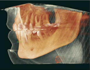
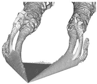
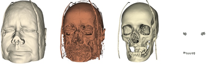
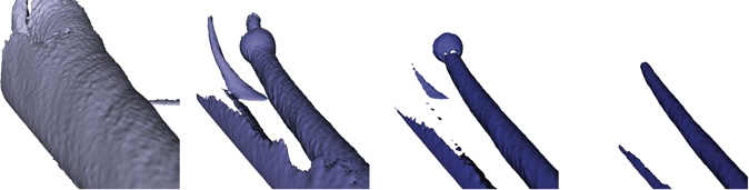
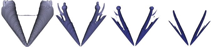
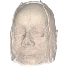
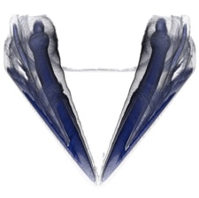
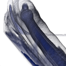
Good volume rendering results depend on the choice of a suitable transfer function. We saw in class that a good transfer function should reveal boundaries present in the volume if such boundaries exist. In the case of globally smooth quantities (such as pressure or vorticity in a CFD simulation) the choice of isovalues aims to reveal important geometric structures in the data. To create such transfer functions for each dataset you will use the code that you wrote for the third assignment to identify important isosurfaces. In the case of the head dataset, salient isosurfaces capture boundaries corresponding to the skin, muscles, skull, and teeth (you saw that the brain is an elusive structure in CT). In the case of the delta wing dataset, you will be looking for isosurfaces that reveal the vortices present on both sides of the wing and in particular the various layers that compose these vortices. Another key feature in this dataset are so-called recirculation bubbles that are present on each side of the trailing edge of the wing (see samples below). Bear in mind that fuzzy structures might be poorly captured by isovalues. Summarize in the report the procedure you followed to find these isovalues for both datasets. Using different opacities for different isosurfaces, create for each dataset a visualization showing all isosurfaces simultaneously.
API specifications: For the sake of simplifying the evaluation of your code, create two executables for this task: salient_medical[.py] and salient_cfd[.py] that each contain the (hardcoded) information needed to visualize the salient isosurfaces of the corresponding dataset using transparency. In both cases, your executable will receive the name of the file to visualize from the command line (which allows us to specify an arbitrary location and resolution for the input file).
Note: Since you are asked to use transparency for this part, refer to the email that was sent recently about the use of depth peeling to obtain correct transparency results in VTK and the specific explanations therein.
Task 2: Transfer function design
Once you have found suitable isovalues, you will design a transfer function for each dataset based upon those values. For that, create a vtkVolumeProperty by following the example provided in Examples/VolumeRendering/*/SimpleRayCast.* to define both color and opacity transfer functions in order to emphasize the selected isovalues. You are already familiar with vtkColorTransferFunctions from previous assignments. The opacity transfer function is defined through a vtkPiecewiseFunction. Your task in designing the opacity transfer function is to reveal as much as possible of the internal structures of each dataset. The volume rendering itself will be performed by raycasting using a vtkVolumeRayCastMapper. Note that this implementation is rather slow but produces very good results. In addition, it takes advantage of the parallelism available on your machine to speed up the computation. Use vtkVolumeRayCastCompositeFunction for value compositing along each ray.
Provide in the report a detailed description of the various transfer functions you created along with a justification of the choices made. What method did you use to create each opacity transfer function? What do you consider to be the strengths and limitations of your solutions?
Create high-quality renderings by combining trilinear interpolation and small sampling distance along each ray. You will need to experiment with different values of the sampling distance to determine the precision necessary to obtain good results. Good results in particular should not exhibit aliasing artifacts such as moiré effect. Note that the value of the sampling distance depends both on the smoothness of the data and on the properties of your transfer function.
API specifications: create two executables dvr_medical[.py] and dvr_cfd[.py] that contain the information necessary to create high quality renderings of the corresponding dataset. In particular, the opacity and color transfer functions must be hard coded in these programs. As for the first task, your executables must obtain the name of the data file from the command line.
Task 3: Volume rendering vs. isosurfacing
Provide for each dataset a side by side comparison between the results obtained for isosurfacing (task 1) and volume rendering (task 2). Make sure to use the same camera settings for both in order to facilitate the comparison. Comment in the report on the differences between the two techniques. Illustrate your argumentation by zooming on particular features of each volume. For each dataset, which technique do you find most effective? Why? Be specific.
Task 4: Multidimensional transfer functions [OPTIONAL: extra credit: 25%]
We saw in class that transfer functions based on value alone may not suffice to properly characterize the boundary of different structures. The third assignment showed for instance that the gradient magnitude offers an additional way to differentiate materials. Following this premise, I am asking you to create a 2D transfer function in which both value and gradient magnitude are used to control the opacity of the volume. For that you will use both the SetScalarOpacity and the SetGradientOpacity functions of the vtkVolumeProperty class. Apply this approach to both datasets and comment in the report on its impact on the resulting visualizations. What are the benefits and the issues associated with this solution? Provide a detailed answer.
Update (4/5/2013)
As we saw in class, vtkVolumeRayCastMapper does not allow you to provide your own precomputed gradient magnitude and instead uses 8-bit precision to compute it internally. This, in turn, requires a downcast from the float precision used to compute the gradient through central differences to the unsigned char precision used for storage of the corresponding magnitude. The solution that I suggested in class consists in precomputing the gradient magnitude through central difference in 8-bit precision and to derive from it the scale and bias parameters used by VTK to do the type conversion. A better solution exists, as it turns out, that was suggested by one of your colleagues and consists in abandoning vtkVolumeRayCastMapper in favor of vtkFixedPointVolumeRayCastMapper.
The key feature of vtkFixedPointVolumeRayCastMapper is its support for so-called multicomponent volumes. While vtkVolumeProperty allows you to define color and opacity for different components (you can supply the index of the component when using SetScalarOpacity or SetColor), vtkFixedPointVolumeRayCastMapper is the only raycasting mapper to actually make use of the information provided for more than one component. Practically, you need to merge the scalar dataset and the gradient magnitude dataset into a single 2-component dataset and then define two opacity transfer function s, one for the first component (index 0, scalar value) and one for the second component (index 1, gradient magnitude). To merge two datasets into a single 2-component dataset you can use vtkImageAppendComponents. Note that another nice feature of vtkFixedPointVolumeRayCastMapper is that you can apply it to datasets of arbitrary types (including float and double). In particular, you can supply a gradient magnitude dataset computed in float precision. There is a caveat however. Internally, the computation will scale the values contained in your data down to 15-bit precision (from 0 to 32768). Regardless, this scaling is done automatically and you can define control points of your opacity transfer function using the original values of your data. In addition, 15-bit precision is much better than the 8-bit precision that vtkVolumeRayCastMapper affords you for the gradient magnitude.
With that in mind, I am giving you the gradient magnitude of both datasets (in small and large resolutions for the visible female) in float and unsigned short precisions. In the case of the unsigned short precision, I have restricted the value range to what I considered to be useful values prior to applying the necessary 16-bit quantization.
Summary Analysis
Provide in the report your critical assessment of volume rendering. What are in your opinion the pros and cons of this technique? Refer to the tasks of this project to justify your opinion.
Data Description
You will be visualizing two datasets for this assignment. The first one is the head CT dataset that you used for the second assignment (see comment below). The second dataset corresponds to a computational fluid dynamics simulation of a delta wing aircraft in a critical flight configuration. In this case the provided scalar volume corresponds to the magnitude of the vorticity, a quantity that is derived from the flow velocity and can be used to identify vortices in numerical datasets.
Note that both datasets have been low-pass filtered (“smoothed”) to facilitate their visualization (e.g., reduce aliasing issues). In particular, the CT dataset in this project is smoother than the one you used previously.
The datasets are available online at http://www.cs.purdue.edu/homes/cs530/Contents/Data/Project4/. All datasets are of type vtkStructuredPoints, which is itself a specialized type of vtkImageData. They are provided in unsigned short (16 bits) precision since this is the highest precision that VTK can volume render using ray casting.
CT dataset
-
-CT scan low resolution (unsigned char, 8.1 MB) (provided for convenience, use the high resolution dataset in your visualizations)
-
-CT scan high resolution (scalar) (unsigned char, 64 MB)
-
-CT gradient high resolution (vector) (float, 383 MB)
-
-CT gradient magnitude high resolution (scalar) (unsigned char, 64 MB)
NEW 04/05/2013:
-
-CT gradient magnitude low resolution (scalar) (float, 17 MB)
-
-CT gradient magnitude low resolution (scalar) (unsigned short, 8 MB, 16-bit quantization was done after clamping the values between 500 and 40,000)
-
-CT gradient magnitude high resolution (scalar) (float, 134 MB)
-
-CT gradient magnitude high resolution (scalar) (unsigned short, 67 MB, 16-bit quantization was done after clamping the values between 1,000 and 40,000)
CFD dataset
-
-vorticity magnitude (scalar) (unsigned short, 18 MB)
-
-gradient of vorticity magnitude (vector) (float, 104 MB)
-
-gradient magnitude of vorticity magnitude (scalar) (unsigned short, 18 MB)
NEW 04/05/2013:
-
-gradient magnitude of vorticity magnitude (scalar) (float, 36 MB)
-
-gradient magnitude of vorticity magnitude (scalar) (unsigned short, 18 MB: 16-bit quantization was done after clamping the values between 1.0e+4 and 2.0e+6)
Sample Images
Following images are meant to provide you with a visual reference for the tasks above. They are by no means a blueprint for what your visualizations should look like.
Task 1.
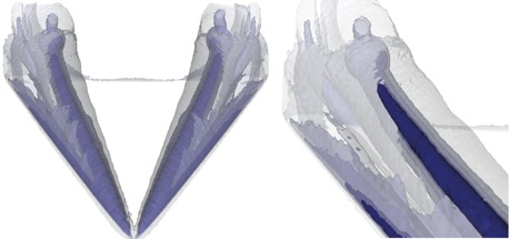
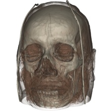
Task 2.
Submission
Submit your solution before March 31 2013 11:59pm using turnin. As a reminder, the submission procedure is as follows.
-
•Include all 4 program files along with any other source code you may have
-
•Include Makefile or CMakeLists.txt file (if applicable). If you are using Visual Studio include the solution file (.sln) and the project files (.vcproj) that are needed to build your project.
-
•Include high resolution sample images showing results for each task
-
•Include a report in HTML OR PDF(*) providing answers to all the questions asked. The report should include mid-res images with links to high-res ones.
-
•Include README.txt file with compilation / execution instructions (optional).
-
•Include all submitted files in a single directory
-
•Do not include binary files
-
•Do not include data files
-
•Do not use absolute paths in your code
After logging into data.cs.purdue.edu, submit your assignment as follows:
% turnin -c cs530 -p project4 <dir_name>
where <dir_name> is the name of the directory containing all your submission material.
Keep in mind that old submissions are overwritten by new ones whenever you execute this command. You can verify the contents of your submission by executing the following command:
% turnin -v -c cs530 -p project4
Do not forget the -v flag here, as otherwise your submission would be replaced by an empty one.
(*) NEW: If you submit your report in PDF format, use cross references in your document to connect the medium size images that you insert in the flow of your text to full resolution images that you place on a separate page, one per page. Make sure to scale the full resolution to its maximal possible size while fitting in the page.