1.1. What are graphs?
A graph is a mathematical structure used to model relationships between objects. It consists of two basic components:
- Nodes (or vertices) — These represent the objects or entities.
- Edges (or links) — These represent the relationships or connections between the objects. The edges can be directed or undirected. In this hand-on lecture, we are going to focus on the undirected graph.

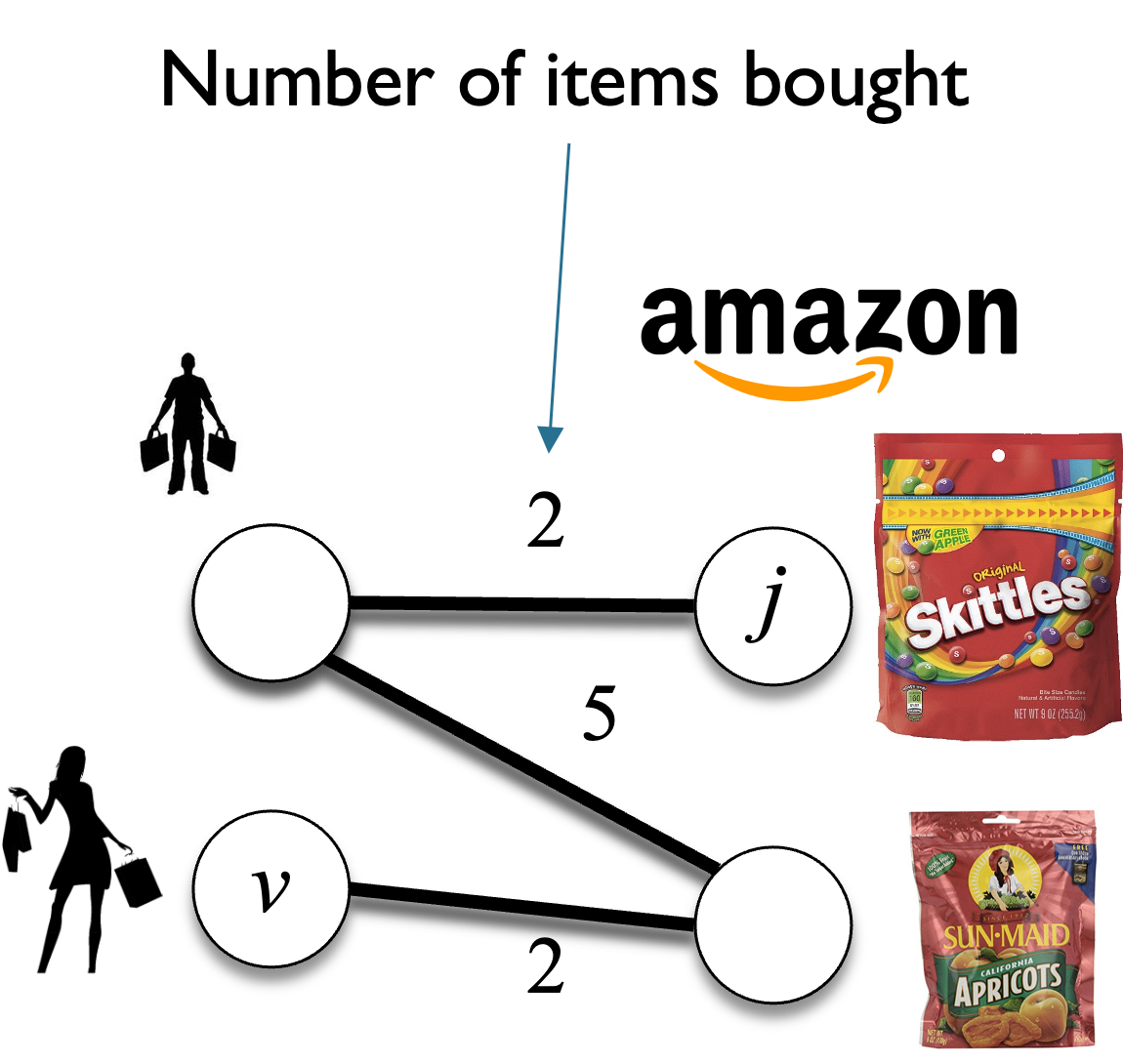
Examples of graphs
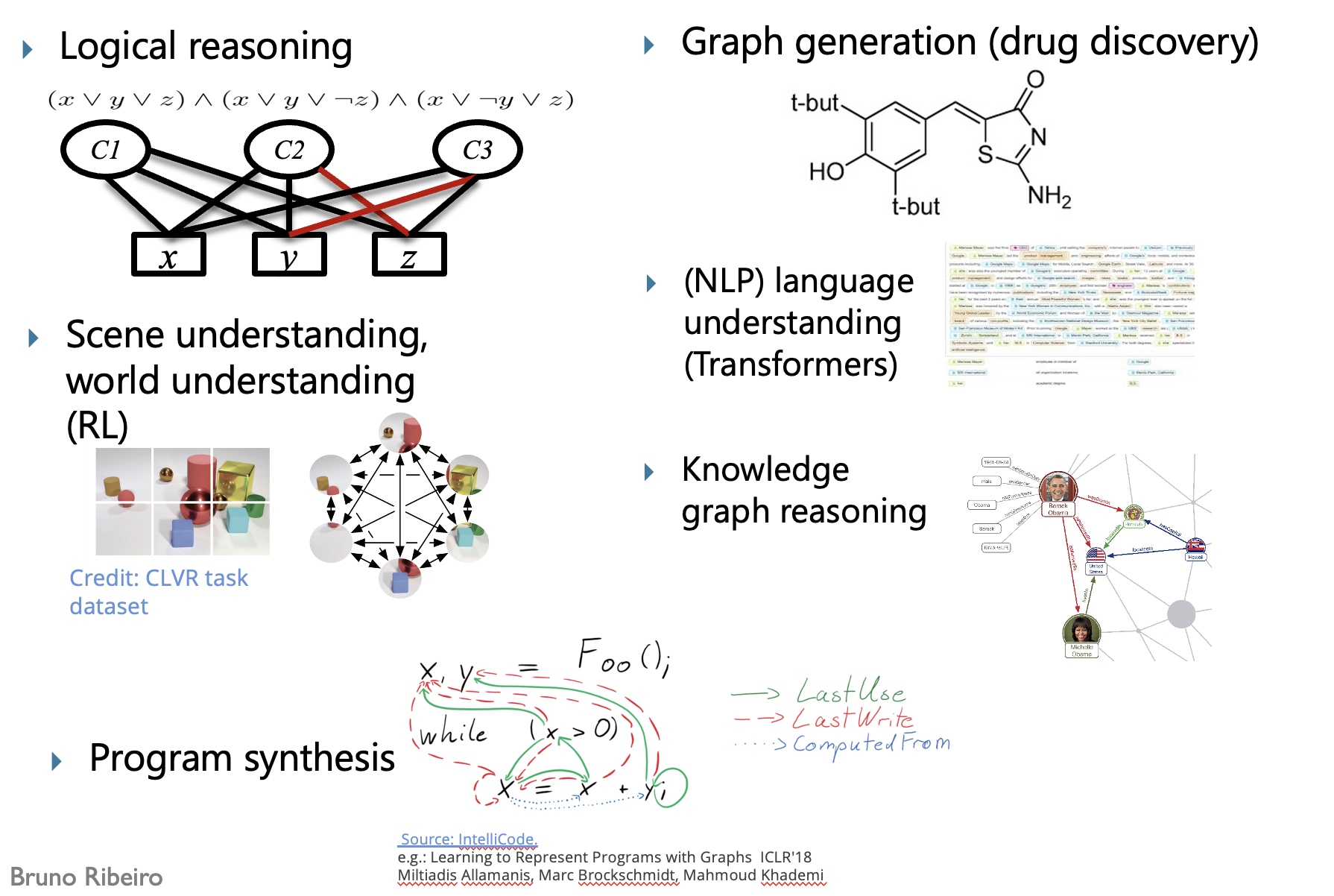
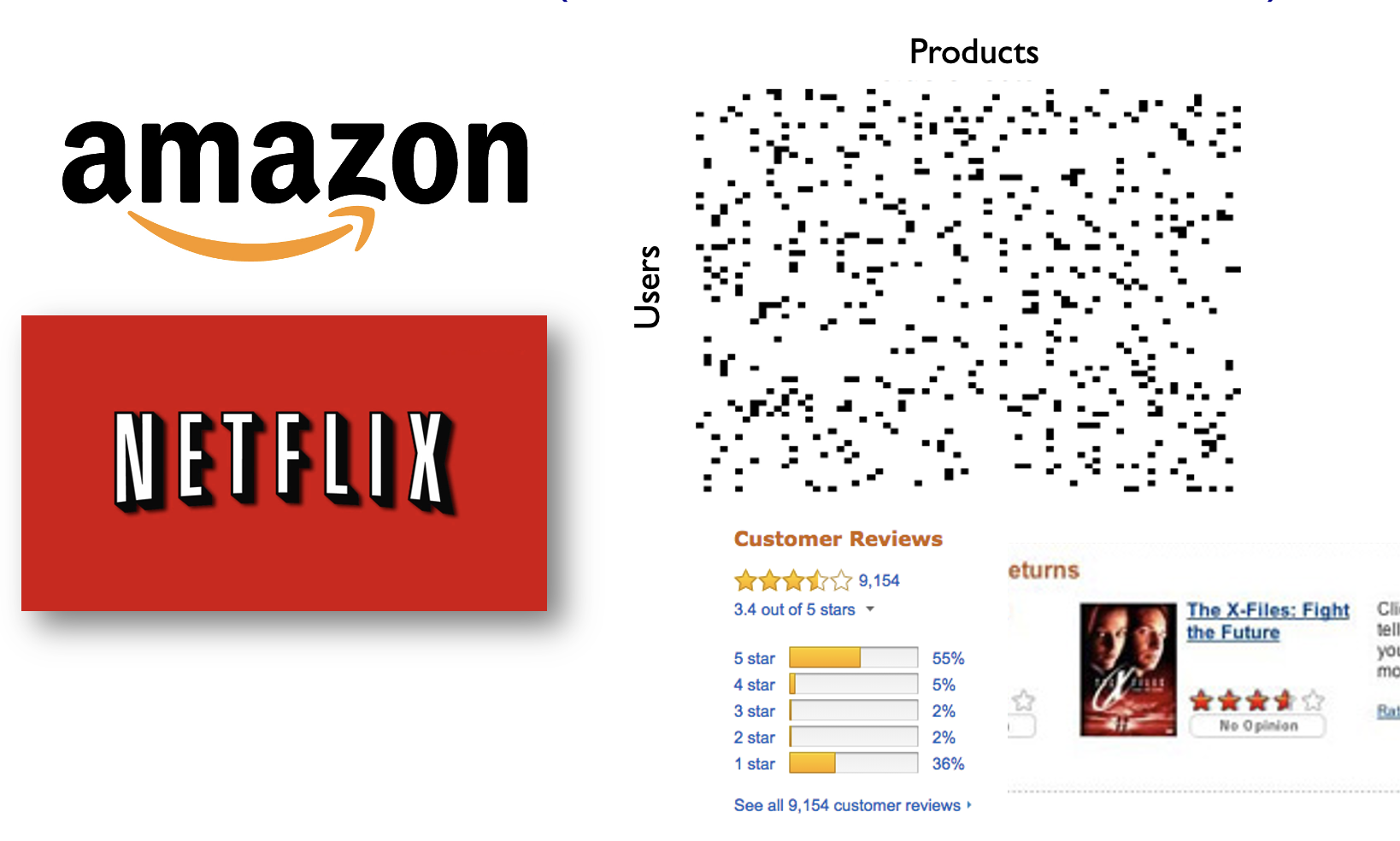
Examples of other graphs
1.2. How to represent vertices and edges in a mathematical way?
The adjacency matrix $A \in \mathbb{A}^{n \times n}$ ($n$ is the number of vertices in the graph) is a square matrix whose elements indicate whether pairs of vertices have a relationship in some appropriate space $\mathbb{A}$.
- In the simplest case, $\mathbb{A} = \{0,1\}$, and $A_{ij} = 1$ if there is a connection from node $i$ to $j$, and otherwise $A_{ij} = 0$ (indicating a non-edge).
- For an undirected graph, keep in mind that $A$ is a symmetric matrix ($A_{ij}=A_{ji}$). For the example graph below has adjacency matrix: $$ A = \begin{bmatrix} 0 & 1 & 0 & 0\\ 1 & 0 & 1 & 1\\ 0 & 1 & 0 & 1\\ 0 & 1 & 1 & 0 \end{bmatrix} $$
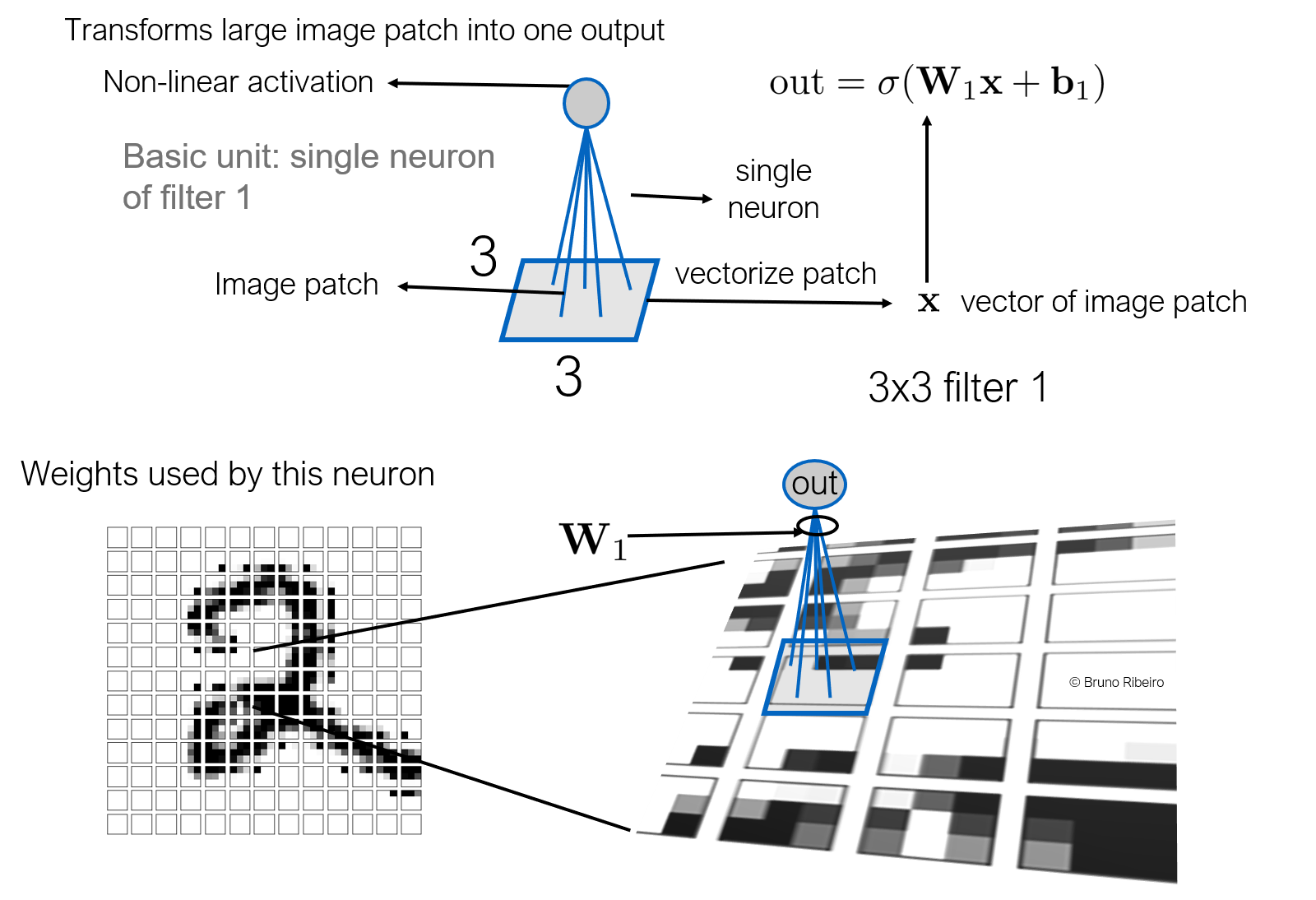
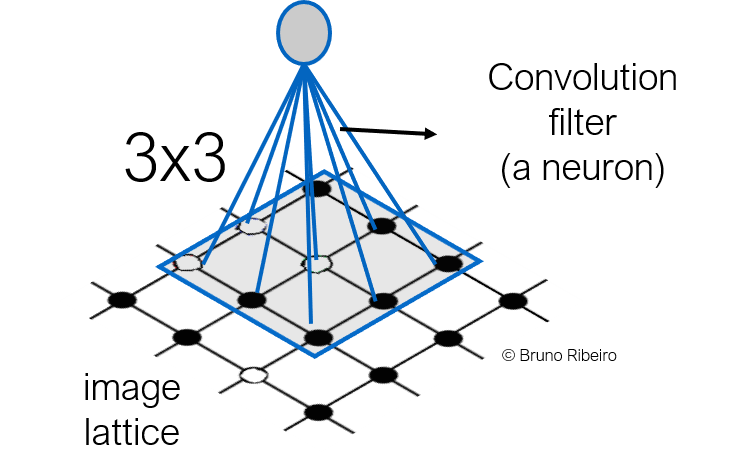
2.1 Images as a lattice
Note that the CNN filter is applied to a constant number of inputs in the last layer.
Topologically, an image is a lattice and the convolution is a filter applied over a patch of the lattice
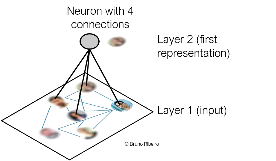
2.2.Feature maps
Then, we apply this convolution in layers, multiple times. Note that each pixel in the previous layer has a convolution representation in the next layer.

2.3. Important to Note
Note that in CNNs:
- Convolutions are applied over fixed-size neighborhoods of a vertex (pixel)
- Convolutions are sensitive to the order of the pixels
Today, we are going to explore convolutions on graphs.

The graph neural layer applied to one of $v$'s friends, say node $u$, will act on $u$'s neighbors (there are four neighbors in $u$'s case).
3.1.1. Challenges of a Graph Convolutions
- Since neighborhoods in a graph can have varying numbers of nodes, Graph Neural Layers cannot use MLPs:
- MLPs and CNN convolutions both take a fixed-size inputs.
- MLPs and CNN convolutions can give different outputs if the order of the inputs change.
3.1.2. Design of the Graph Neural Layer
- A Graph Neural Network (GNN) is similar to a Convolution Neural Network except that
- GNN convolutions can take variable-size inputs.
- GNN convolutions can give the same outputs if the order of the inputs change.
Definition: (Representations) We will call a vector ${\bf h}$ a representation if it is composed of neuron outputs.
- In a GNN, each node in the graph gets its own representation at each GNN layer:
- The graph is defined by its set of nodes $V$ and set of edges $E$. Graph $G$ is denoted $G=(V,E)$.
- At layer $k$ of a GNN, ${\bf h}^{(k)}_v \in \mathbb{R}^{1 \times d}$, $d \geq 1$, will denote the representation of node $v \in V$ at layer $k$ of the GNN.
The $k$-th representation ${\bf h}^{(k)}_v \in \mathbb{R}^{1 \times d_k}$, $d_k \geq 1$ of node $v \in V$ can be described through:
- Node $v$'s own representation at layer $k-1$, ${\bf h}^{(k-1)}_v \in \mathbb{R}^{1 \times d_{k-1}}$, $d_{k-1}$ is the representation size of the previous GNN layer and
- The representations of its neighbors ${\bf h}^{(k-1)}_u$, $\forall u \in \mathcal{N}_v$, where $\mathcal{N}_v$ is the set of neighbors of $v$ in the graph $G$.
Here:
- ${\bf h}^{(k)}_v$ is how layer $k$ represents node $v$. It is a $1 \times d_k$ vector.
- Note that $d_k$ may be different from $d_{k-1}$.
3.1.3. Graph Neural Layer: Represenation of node v at layer k
Here, we describe how combine representations of node $v$ and its neighbors at layer $k-1$ to get represenation of node $v$ at layer $k$. $$ {\bf h}^{(k)}_v = \sigma\left( {\bf h}^{(k-1)}_v {\bf W}_\text{self}^{(k)} + \sum_{\forall u \in \mathcal{N}_v} {\bf h}^{(k-1)}_u {\bf W}_\text{neig}^{(k)} + {\bf b}^{(k)} \right), $$ where ${\bf W}_\text{self}^{(k)} \in \mathbb{R}^{d' \times d}$, ${\bf W}_\text{neigh}^{(k)} \in \mathbb{R}^{d' \times d}$, ${\bf b}^{(k)} \in \mathbb{R}^{1 \times d}$, $d'\in \mathbb{N}$ and $\mathcal{N}_v$ are the neighbors of node $v$ in the graph.
Here:
- ${\bf W}_\text{self}^{(k)} \in \mathbb{R}^{d' \times d}$, ${\bf W}_\text{neigh}^{(k)} \in \mathbb{R}^{d' \times d}$, and $b$ are learnable parameters.
- $\sigma$ is the activation function.
The below image illustrates the equation by:
- Graph Structure: Shows node $ v $ at layer $ k $ with neighbors $ u_1 $ and $ u_2 $ at layer $ k-1 $.
- Formula Breakdown: Calculates $ h_v^{(k)} $ step-by-step:
- Self-representation $ h_v^{(k-1)} W_{\text{self}}^{(k)} $.
- Neighbor sum $ \sum h_u^{(k-1)} W_{\text{neigh}}^{(k)} $.
- Adds bias $ b^{(k)} $.
- Applies activation $ \sigma $ (ReLU here).
This shows how node $ v $'s representation is computed by combining info from itself and neighbors.

3.2.2. Creating the graph
import torch
import torch.nn as nn
import numpy as np
import networkx as nx

torch.manual_seed(13)

# Graph initialization

input_features = {
    'White Spruce':  torch.tensor([1, .5, 0],dtype=torch.float32),
    'Snowshoe Hare': torch.tensor([1, .5, 0],dtype=torch.float32),
    'Red Squirrel': torch.tensor([1, .5, 0],dtype=torch.float32),
    'Ground Squirrel': torch.tensor([1, .5, 0],dtype=torch.float32),
    'Coyote': torch.tensor([1, .5, 0],dtype=torch.float32),
    'Red Fox': torch.tensor([1, .5, 0],dtype=torch.float32),
    'Lynx': torch.tensor([1, .5, 0],dtype=torch.float32)
}

targets = {
    'White Spruce': 0,
    'Snowshoe Hare': 0,
    'Red Squirrel': 0,
    'Ground Squirrel': 0,
    'Coyote': 1,
    'Red Fox': 1,
    'Lynx': 1
}

edges = [
    ('White Spruce', 'Snowshoe Hare'),
    ('White Spruce', 'Red Squirrel'),
    ('Snowshoe Hare', 'Red Squirrel'),
    ('Snowshoe Hare', 'Ground Squirrel'),
    ('Snowshoe Hare', 'Coyote'),
    ('Snowshoe Hare', 'Red Fox'),
    ('Ground Squirrel', 'Lynx'),
    ('Red Squirrel', 'Coyote'),
    ('Red Squirrel', 'Lynx'),
    ('Coyote', 'Lynx'),
    ('Ground Squirrel', 'Coyote'),
    ('Red Fox', 'Lynx')
]

G = nx.Graph()
G.add_edges_from(edges)
3.2.2. Defining the GNN Layer
- We now define a GNNLayer, which is a single layer of a GNN
- It looks a lot like defining a convolutional layer for a CNN
PS: Please download the library mygraphlib.py and put in the same folder as this notebook
import torch
import torch.nn as nn
import torch.nn.functional as F
# import some useful functions for this notebook
import mygraphlib as mylib

class GNNLayer(nn.Module):
    def __init__(self, input_dim, output_dim):
        super(GNNLayer, self).__init__()
        # We will define the parameters differently this time
        self.W_self = nn.Parameter(torch.Tensor(input_dim, output_dim))
        self.W_agg = nn.Parameter(torch.Tensor(input_dim, output_dim))
        nn.init.xavier_uniform_(self.W_self)
        nn.init.xavier_uniform_(self.W_agg)

    def forward(self, h, A):
        new_h_self = h @ self.W_self
        new_h_agg = (A @ h) @ self.W_agg
        return F.leaky_relu(new_h_self + new_h_agg)
3.2.3. Data Preparation
- We first move all the data into torch.tensor objects
# Aata preparation
node_order = list(input_features.keys())
node_features = torch.stack([input_features[node] for node in node_order])
# Define the adjacency matrix
A = nx.to_numpy_array(G, nodelist=node_order)
A = torch.tensor(A, dtype=torch.float32)
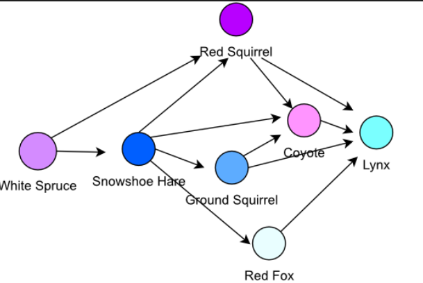
mylib.visualize_graph(G, node_features, title=f'Input Graph',mycmap="Spectral")
/Users/ribeirob/anaconda3/envs/cs373/lib/python3.11/site-packages/networkx/drawing/nx_pylab.py:450: UserWarning: No data for colormapping provided via 'c'. Parameters 'cmap' will be ignored
  node_collection = ax.scatter(

3.2.3. Showing the ouput of the first GNN Layer
This is the output of applying the first GNN layer
- Since the node representations in layer 1 have dimension $d_1 = 3$, we can visualize them normalized as RGB colors.
- Can you find the nodes that have the same representations?
- Why do they have the same representations?
# Instantiate a GNN layer
gnn_layer = GNNLayer(input_dim=3, output_dim=3)

# We will now apply the first layer
layer = 1

# Dictionary to store all representations of the nodes
# h[0] are the initial node features
h = {0:node_features}

h[layer] = gnn_layer(h[layer-1], A)

mylib.visualize_graph(G, h[layer], title=f'Graph After Layer {layer}',mycmap="Spectral")

Let's apply the same GNN layer again
- Since the node representations in layer 2 have dimension $d_2 = 3$, we can visualize them normalized as RGB colors.
- Can you find the nodes that have the same representations?
- Why do they have the same representations?
# Apply another layer of the GNN
layer += 1

h[layer] = gnn_layer(h[layer-1], A)

mylib.visualize_graph(G, h[layer], title=f'Graph After Layer {layer}',mycmap="Spectral")

Let's apply the same GNN layer again
- Since the node representations in layer 3 have dimension $d_3 = 3$, we can visualize them normalized as RGB colors.
- Can you find the nodes that have the same representations?
- Why do they have the same representations?
# Apply another layer of the GNN
layer += 1

h[layer] = gnn_layer(h[layer-1], A)

mylib.visualize_graph(G, h[layer], title=f'Graph After Layer {layer}',mycmap="Spectral")

Let's apply the same GNN layer again
- Since the node representations in layer 2 have dimension $d_2 = 3$, we can visualize them normalized as RGB colors.
- Now no nodes have the same representation
- Why do they get different representations?
# Apply another layer of the GNN
layer += 1

h[layer] = gnn_layer(h[layer-1], A)

mylib.visualize_graph(G, h[layer], title=f'Graph After Layer {layer}',mycmap="Spectral")

3.3. Model search on the GNN (GNN training)
- We are going to build a GNN with:
- four GNN layers that output to
- an MLP with one hidden layer
- which ten outputs a single probability (large or small animal)
- After the model is trained, we will use the model to predict new data points. Let's first train the model.
import torch
import torch.nn as nn
import torch.optim as optim
import torch.nn.functional as F
import networkx as nx


class myGNN(nn.Module):
    def __init__(self, input_dim, hidden_dim, output_dim, mlp_hidden_dim):
        super(myGNN, self).__init__()
        self.gnn_layer1 = GNNLayer(input_dim, hidden_dim)
        self.gnn_layer2 = GNNLayer(hidden_dim, hidden_dim)
        self.gnn_layer3 = GNNLayer(hidden_dim, hidden_dim)
        self.gnn_layer4 = GNNLayer(hidden_dim, hidden_dim)

        self.mlp_layer1 = nn.Linear(hidden_dim, mlp_hidden_dim)
        self.mlp_layer2 = nn.Linear(mlp_hidden_dim, output_dim)

    def forward(self, node_features, A):
        h = self.gnn_layer1(node_features, A)
        h = self.gnn_layer2(h, A)
        h = self.gnn_layer3(h, A)
        h = self.gnn_layer4(h, A)

        h = F.relu(self.mlp_layer1(h))
        h = torch.sigmoid(self.mlp_layer2(h))
        return h
node_order = list(input_features.keys())
node_features = torch.stack([input_features[node] for node in node_order])
# Adjacency matrix
A = nx.to_numpy_array(G, nodelist=node_order)
A = torch.tensor(A, dtype=torch.float32)
labels = torch.tensor([targets[node] for node in node_order], dtype=torch.float32).unsqueeze(1)
input_dim = 3
hidden_dim = 100
mlp_hidden_dim = 100
output_dim = 1

model = myGNN(input_dim, hidden_dim, output_dim, mlp_hidden_dim)
loss_function = nn.BCELoss()
optimizer = optim.Adam(model.parameters(), lr=0.001)

epochs = 1000
model.train()
for epoch in range(epochs):

    predictions = model(node_features, A)

    loss = loss_function(predictions, labels)

    optimizer.zero_grad()
    loss.backward()
    optimizer.step()

    if epoch % 100 == 0:
        print(f'Epoch {epoch}, Loss: {loss.item()}')

print(f'Epoch {epoch}, Loss: {loss.item()}')
Epoch 0, Loss: 0.6811298131942749
Epoch 100, Loss: 0.6795715093612671
Epoch 200, Loss: 0.6881592869758606
Epoch 300, Loss: 0.47657492756843567
Epoch 400, Loss: 0.019529860466718674
Epoch 500, Loss: 0.0014836833579465747
Epoch 600, Loss: 0.00043085546349175274
Epoch 700, Loss: 5.011613029637374e-05
Epoch 800, Loss: 2.352609226363711e-05
Epoch 900, Loss: 1.4463118532148656e-05
Epoch 999, Loss: 1.0031370038632303e-05
Now let's use the model to predict all data points in the training set to calculate a train accuracy.
model.eval()
correct_predictions = 0

with torch.no_grad():
    model.eval()
    train_predictions = model(node_features, A)
    for i, prediction in enumerate(train_predictions):
        true_label = labels[i].item()
        predicted_class = 'big' if prediction.item() > 0.5 else 'small'
        predicted_class_label = 1 if prediction.item() > 0.5 else 0
        true_class = 'big' if true_label == 1 else 'small'
        if predicted_class_label == true_label:
            correct_predictions += 1
        print(f".. {node_order[i]}: True = {true_class}, Predicted = {predicted_class}, Probability = {prediction.item():.4f}")

train_accuracy = correct_predictions / len(node_order) * 100
print(f"\nTraining Accuracy: {train_accuracy:.2f}%")
.. White Spruce: True = small, Predicted = small, Probability = 0.0000
.. Snowshoe Hare: True = small, Predicted = small, Probability = 0.0000
.. Red Squirrel: True = small, Predicted = small, Probability = 0.0000
.. Ground Squirrel: True = small, Predicted = small, Probability = 0.0000
.. Coyote: True = big, Predicted = big, Probability = 1.0000
.. Red Fox: True = big, Predicted = big, Probability = 1.0000
.. Lynx: True = big, Predicted = big, Probability = 1.0000

Training Accuracy: 100.00%
3.3.2. Testing the trained GNN model
It seems that our model perfectly fit the train set. But how about on a new graph with new data points?
new_G = nx.Graph()

new_edges = [
    ('Bear', 'Deer'),
    ('Deer', 'Raccoon'),
    ('Raccoon', 'Hedgehog'),
    ('Hedgehog', 'Rabbit'),
    ('Rabbit', 'Wolf'),
    ('Wolf', 'Bear'),
    ('Bear', 'Rabbit')
]
new_G.add_edges_from(new_edges)

new_input_features = {
    'Bear': torch.tensor([1,0.5,0]),
    'Deer': torch.tensor([1,0.5,0]),
    'Raccoon': torch.tensor([1,0.5,0]),
    'Hedgehog': torch.tensor([1,0.5,0]),
    'Rabbit': torch.tensor([1,0.5,0]),
    'Wolf': torch.tensor([1,0.5,0]),
}

new_targets = {
    'Bear': 1,
    'Deer': 1,
    'Raccoon': 0,
    'Hedgehog': 0,
    'Rabbit': 0,
    'Wolf': 1
}

new_node_order = list(new_input_features.keys())
new_node_features = torch.stack([new_input_features[node] for node in new_node_order])

new_adj_matrix = nx.to_numpy_array(new_G, nodelist=new_node_order)
new_adj_matrix = torch.tensor(new_adj_matrix, dtype=torch.float32)

model.eval()
correct_predictions = 0

with torch.no_grad():
    new_predictions = model(new_node_features, new_adj_matrix)

    for i, prediction in enumerate(new_predictions):
        predicted_class = 'big' if prediction.item() > 0.5 else 'small'
        predicted_class_label = 1 if prediction.item() > 0.5 else 0
        true_label = new_targets[new_node_order[i]]

        if predicted_class_label == true_label:
            correct_predictions += 1

        print(f"New Node {new_node_order[i]}: True = {'big' if true_label == 1 else 'small'}, "
              f"Predicted = {predicted_class}, Probability = {prediction.item():.4f}")

test_accuracy = correct_predictions / len(new_node_order) * 100
print(f"\nTest Accuracy: {test_accuracy:.2f}%")
New Node Bear: True = big, Predicted = small, Probability = 0.0015
New Node Deer: True = big, Predicted = big, Probability = 1.0000
New Node Raccoon: True = small, Predicted = small, Probability = 0.0122
New Node Hedgehog: True = small, Predicted = big, Probability = 1.0000
New Node Rabbit: True = small, Predicted = small, Probability = 0.0015
New Node Wolf: True = big, Predicted = big, Probability = 1.0000

Test Accuracy: 66.67%
4. (Extra) Edge (link) prediction using GNNs
It generalizes well! Now, let's try to do edge prediction. Link prediction in a graph refers to predicting whether an edge exists between two nodes based on their node features and the structure of the graph. GNNs can be used for this by learning embeddings for nodes and then using these embeddings to predict edges.
Specifically, here is how we do it:
- The GNN model learns a representation for each node based on its features and the graph structure.
Predicting missing edges:
- For each pair of nodes, combine their embeddings to compute the likelihood of an edge. This can be done using techniques such as concatenation, element-wise multiplication, or a distance function (e.g., cosine similarity, dot product).
- Apply a classifier or a score function to the combined node embeddings to predict whether an edge exists between the nodes.
Now, we will combine node embeddings from our trained GNN with element-wise multiplication and use that as edge representation. We are going to train a MLP on the train data we have to predict whether an edge exist based on the edge representation. Finally, we are going to apply that link predictor to the test data.
node_order_train = list(input_features.keys())
node_features_train = torch.stack([input_features[node] for node in node_order_train])
adj_matrix_train = nx.to_numpy_array(G, nodelist=node_order_train)
adj_matrix_train = torch.tensor(adj_matrix_train, dtype=torch.float32)

class LinkPredictor(nn.Module):
    def __init__(self, input_dim):
        super(LinkPredictor, self).__init__()
        self.fc1 = nn.Linear(input_dim, 8)
        self.fc2 = nn.Linear(8, 1)

    def forward(self, x):
        x = F.relu(self.fc1(x))
        x = torch.sigmoid(self.fc2(x))
        return x

def get_node_embeddings(model, node_features, adj_matrix):
    model.eval()
    with torch.no_grad():
        node_embeddings = model.gnn_layer1(node_features, adj_matrix)
        node_embeddings = model.gnn_layer2(node_embeddings, adj_matrix)
    return node_embeddings

def prepare_edge_prediction_data_with_labels(G, node_embeddings, node_order):
    edges = list(G.edges())
    non_edges = list(nx.non_edges(G))

    data = []
    labels = []

    for (node1, node2) in edges:
        combined_embedding = node_embeddings[node_order.index(node1)] * node_embeddings[node_order.index(node2)]
        data.append(combined_embedding)
        labels.append(1)

    for (node1, node2) in non_edges:
        combined_embedding = node_embeddings[node_order.index(node1)] * node_embeddings[node_order.index(node2)]
        data.append(combined_embedding)
        labels.append(0)
    data = torch.stack(data)
    labels = torch.tensor(labels, dtype=torch.float32).unsqueeze(1)
    return data, labels

predictor = LinkPredictor(hidden_dim)
optimizer = optim.Adam(predictor.parameters(), lr=0.01)
loss_function = nn.BCELoss()
node_embeddings_train = get_node_embeddings(model, node_features_train, adj_matrix_train)

train_data, train_labels = prepare_edge_prediction_data_with_labels(G, node_embeddings_train, node_order_train)

epochs = 100
for epoch in range(epochs):
    predictor.train()
    predictions = predictor(train_data)
    loss = loss_function(predictions, train_labels)
    optimizer.zero_grad()
    loss.backward()
    optimizer.step()

    if epoch % 10 == 0:
        print(f"Epoch {epoch}, Loss: {loss.item():.4f}")

predictor.eval()
with torch.no_grad():
    predictions_train = predictor(train_data)
    predicted_labels_train = (predictions_train > 0.5).float()
    correct_predictions = (predicted_labels_train == train_labels).float().sum()
    train_accuracy = correct_predictions / len(train_labels) * 100
    print(f"Training Accuracy: {train_accuracy:.2f}%")
Epoch 0, Loss: 0.8903
Epoch 10, Loss: 0.6508
Epoch 20, Loss: 0.6288
Epoch 30, Loss: 0.5989
Epoch 40, Loss: 0.5753
Epoch 50, Loss: 0.5554
Epoch 60, Loss: 0.5348
Epoch 70, Loss: 0.5135
Epoch 80, Loss: 0.4910
Epoch 90, Loss: 0.4664
Training Accuracy: 80.95%
Now let's this simple link predictor on the test set. The results are not very good. Probability due to:
- The model architecture too simple.
- The predator-prey relationship is much more complex to model than size.
- Too few data points.
new_G = nx.Graph()
new_G.add_edges_from(new_edges)

node_order_new = list(new_input_features.keys())
new_node_features = torch.stack([new_input_features[node] for node in node_order_new])
new_adj_matrix = nx.to_numpy_array(new_G, nodelist=node_order_new)
new_adj_matrix = torch.tensor(new_adj_matrix, dtype=torch.float32)

new_node_embeddings = get_node_embeddings(model, new_node_features, new_adj_matrix)
new_data, new_labels = prepare_edge_prediction_data_with_labels(new_G, new_node_embeddings, node_order_new)

predictor.eval()
with torch.no_grad():
    new_predictions = predictor(new_data)
    predicted_labels_new = (new_predictions > 0.5).float()

print("Predictions for new graph edges:")
correct_predictions = 0

all_edges = list(new_G.edges()) + list(nx.non_edges(new_G))
for i, (node1, node2) in enumerate(all_edges):
    predicted_class = "edge" if predicted_labels_new[i].item() == 1 else "no edge"
    ground_truth_class = "edge" if new_labels[i].item() == 1 else "no edge"

    if predicted_labels_new[i].item() == new_labels[i].item():
        correct_predictions += 1

    print(f"Edge between {node1} and {node2}: Predicted = {predicted_class}, Ground Truth = {ground_truth_class}")

test_accuracy = correct_predictions / len(new_labels) * 100
print(f"\nTest Accuracy: {test_accuracy:.2f}%")
Predictions for new graph edges:
Edge between Bear and Deer: Predicted = no edge, Ground Truth = edge
Edge between Bear and Wolf: Predicted = no edge, Ground Truth = edge
Edge between Bear and Rabbit: Predicted = no edge, Ground Truth = edge
Edge between Deer and Raccoon: Predicted = no edge, Ground Truth = edge
Edge between Raccoon and Hedgehog: Predicted = no edge, Ground Truth = edge
Edge between Hedgehog and Rabbit: Predicted = no edge, Ground Truth = edge
Edge between Rabbit and Wolf: Predicted = no edge, Ground Truth = edge
Edge between Rabbit and Deer: Predicted = no edge, Ground Truth = no edge
Edge between Rabbit and Raccoon: Predicted = no edge, Ground Truth = no edge
Edge between Deer and Wolf: Predicted = no edge, Ground Truth = no edge
Edge between Deer and Hedgehog: Predicted = no edge, Ground Truth = no edge
Edge between Hedgehog and Wolf: Predicted = no edge, Ground Truth = no edge
Edge between Hedgehog and Bear: Predicted = no edge, Ground Truth = no edge
Edge between Wolf and Raccoon: Predicted = no edge, Ground Truth = no edge
Edge between Raccoon and Bear: Predicted = no edge, Ground Truth = no edge

Test Accuracy: 53.33%