What is Backpropagation?
- Backpropagation is an algorithm used for computing gradients of the parameters of a neural network with respect to a loss function.
- It computes the gradient of the loss function with respect to each weight by propagating the error backward through the network, using the chain rule to update the weights in proportion to the error's gradient.
- a univariate (non-polynomial) activation function, denoted $\sigma : \mathbb{R} \to \mathbb{R}$,
- a (column) vector of weights, denoted ${\bf w} = (w_1, \ldots, w_n) \in \mathbb{R}^n$, and
- a threshold (bias) value, denoted $b \in \mathbb{R}$.
Given an input vector ${\bf x} = (x_l, \ldots , x_n)$ is fed into the neuron through the input units, the neuron function computes $h({\bf x}) = \sigma({\bf w}^T {\bf x} + b)$. The value of this function is the neuron's output.
Gradient Descent: General Recursive Gradient Computation (Backpropagation)
Recap: Feedforward neural network (FFNN a.k.a. MLP)
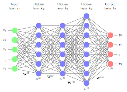
The general architecture of a feedforward neural network is:
- an input layer with $n$ input-units
- an output layer with $m$ outputs
- and one or more hidden layers consisting of intermediate neuron outputs.
- the superscript $(k)$ in the parameters (weights) ${\bf W}^{(k)}$ will indicate they belong to layer $k$
- if layer $k$ has $d_\text{in}$ inputs and $d_\text{out}$ outputs, then the neuron weights ${\bf W}^{(k)}\in \mathbb{R}^{n_\text{in} \times n_\text{out}}$ are a $n_\text{in} \times n_\text{out}$ matrix
The maximum log-likelihood optimization will use gradient ascent:
Let ${\bf W} = ({\bf w}^{(1)},{\bf w}^{(2)},{\bf w}^{(3)})$.
Obtaining ${\bf W}$ via maximum likelihood estimation using gradient ascent.
Let $\text{Data} = \{({\bf x}(i),y(i))\}_{i=1}^n$
$$\begin{align*}
&\frac{\partial}{\partial {\bf W}} \text{log-likelihood(Data)} = \frac{\partial}{\partial {\bf W}} \sum_{i=1}^n \log p(y = y(i) | {\bf x}(i); {\bf w}^{(1)}, {\bf w}^{(2)}, {\bf w}^{(3)} ) \\
&= \sum_{i=1}^n y(i) \frac{\partial}{\partial {\bf W}} \log \sigma(({\bf w}^{(3)})^T {\bf h}({\bf x}(i))) + (1 - y(i)) \frac{\partial}{\partial {\bf W}} \log (1-\sigma(({\bf w}^{(3)})^T {\bf h}({\bf x}(i)))) \\
\end{align*}
$$
where $\sigma(x) = \frac{\exp(x)}{1 + \exp(x)}$, and ${\bf h}({\bf x}) = (1,\hat{h}_1({\bf x}),\hat{h}_2({\bf x}))$,
$$
\hat{h}_1({\bf x}) = p(h_1 = 1 | {\bf x}) = \sigma(({\bf w}^{(1)})^T {\bf x})
$$
and
$$
\hat{h}_2({\bf x}) = p(h_2 = 1 | {\bf x}) = \sigma(({\bf w}^{(2)})^T {\bf x})
$$
How can we compute these gradients? Here, we will resort to the chain rule of vector Calculus.
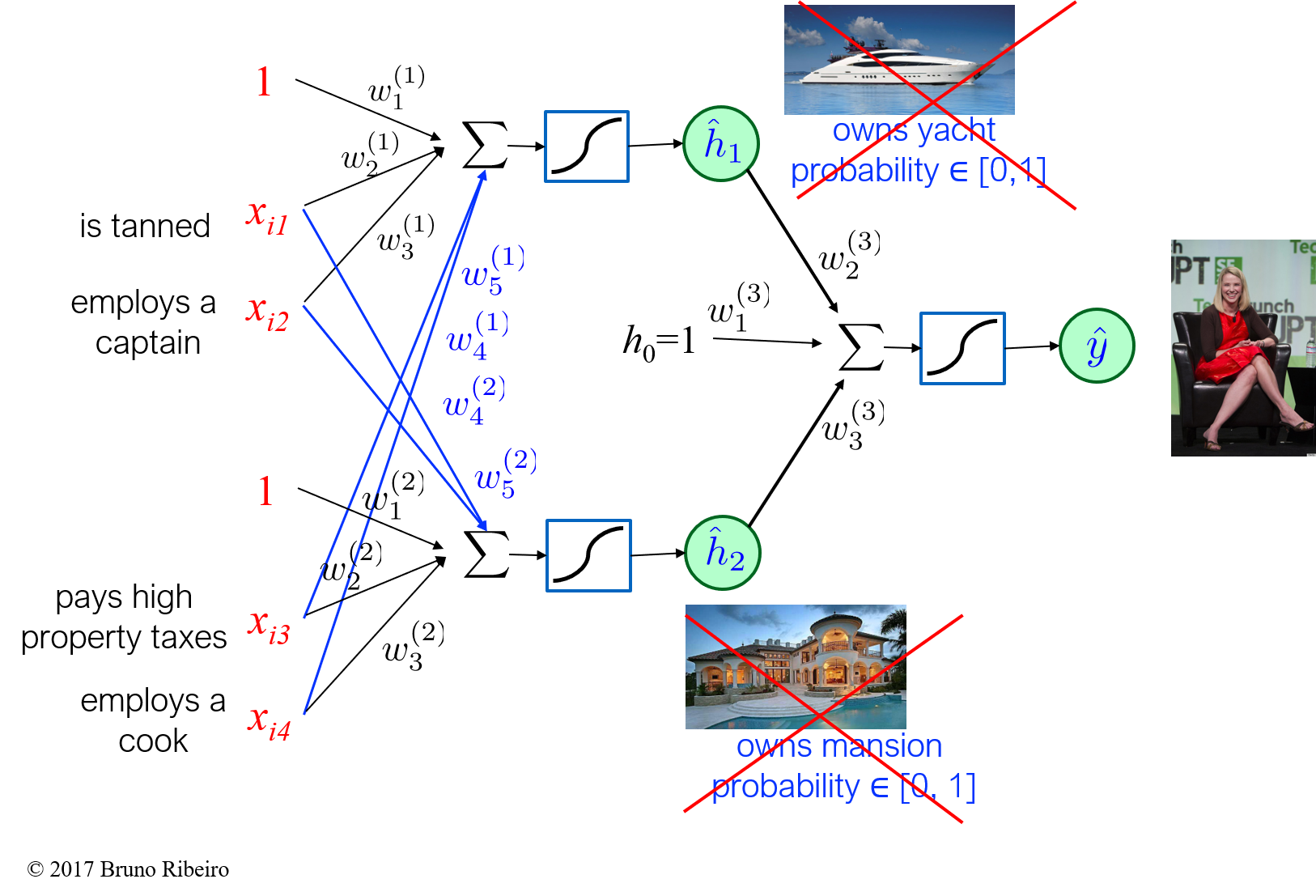
In a deep neural network each layer is a composition of previous layers, in our previous example the composition looks like:
 defined as
$$f^1({\bf x};{\bf w}^{(1)}) = \sigma(({\bf w}^{(1)})^T {\bf x}), $$
and
$$f^2({\bf h};{\bf w}^{(3)}) = \sigma(({\bf w}^{(3)})^T {\bf h}) ,$$
where $\hat{{\bf h}} = (1,\hat{h}_1,\hat{h}_2)$.
defined as
$$f^1({\bf x};{\bf w}^{(1)}) = \sigma(({\bf w}^{(1)})^T {\bf x}), $$
and
$$f^2({\bf h};{\bf w}^{(3)}) = \sigma(({\bf w}^{(3)})^T {\bf h}) ,$$
where $\hat{{\bf h}} = (1,\hat{h}_1,\hat{h}_2)$.
The derivative of the composition $f^2(f^1(x;{\bf w}^{(1)});{\bf w}^{(3)})$ with respect to ${\bf w}^{(1)}_2$ is $$ \frac{\partial f^2(f^1(x;{\bf w}^{(1)});{\bf w}^{(3)})}{\partial {\bf w}^{(1)}_2} = \frac{\partial f^2({\bf h})}{\partial {\bf h}} \bigg|_{h = f^1({\bf x};{\bf w}^{(1)})} \cdot \frac{\partial f^1({\bf x};{\bf w}^{(1)})}{\partial {\bf w}_2^{(1)}}. $$
General solution: Consider having $K > 1$ hidden layers. The influence of a lower layer parameter in the final error can be recovered by the chain rule, which generally states:
$$ \frac{\partial f^K(f^{K-1}(\cdots f^2(f^1(x;{\bf w}^{(1)}))\cdots))}{\partial {\bf w}^{(1)}_2} = \frac{\partial f^K(f^{K-1})}{\partial f^{K-1}} \cdot \frac{\partial f^{K-1}(f^{K-2})}{\partial f^{K-2}} \cdots \frac{\partial f^2(f^1)}{\partial f^1} \cdot \frac{\partial f^1({\bf x};{\bf w}^{(1)})}{\partial {\bf w}_2^{(1)}}. $$
General Recursive Gradient Computation (Backpropagation)
More generally, for deep neural networks we have no hope of writing down gradient formula for all parameters. We need a recursive method.
- backpropagation = recursive application of the chain rule along a computational graph to compute the gradients of all inputs/parameters/intermediates
- Widely used implementations maintain a graph structure, where the nodes implement the forward() / backward() functions.
- forward pass: compute result of an operation and save any intermediates needed for gradient computation in memory
- backward pass: apply the chain rule to compute the gradient of the loss function with respect to the inputs.
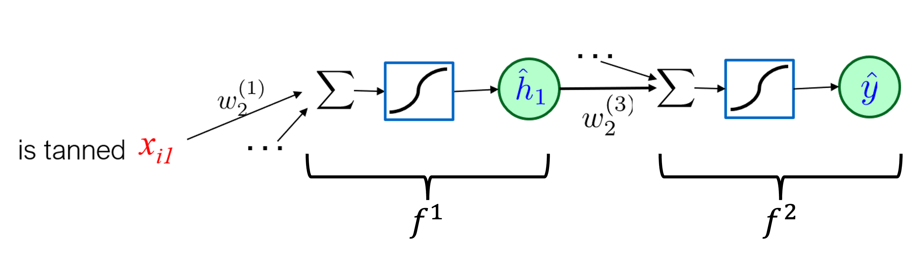
The recursion can be explained with a single image. Consider the following general algorithm to recursively compute the gradient:
- The activations of the hidden neurons are given by $\hat{{\bf h}}^{(k)} = (1,\sigma({\bf W}_k \hat{{\bf h}}^{(k-1)}))$, $k=1,\ldots,K$, where
- The input is $\hat{{\bf h}}^{(0)} = ({\bf x},1)$, where ${\bf x}$ is a single training example.
- And the operator $(1,{\bf z})$ concatenates $1$ to vector ${\bf z}$.
- $L(\hat{{\bf h}}^{(K)})$ is the log-likelihood of a single example. If we consider multiple training examples $\{{\bf x}_1,\ldots,{\bf x}_N\}$, we have the loss over $L(\{\hat{{\bf h}}^{(K)}(i)\}_{i=1}^N)$, which is the sum of the losses over each individual training example.
Backpropagation: Practical Challenges with Deep Models
Quiz 1: Understanding backpropagation as an algorithm that is called up to $K$ times, recursively, to multiplies gradients, what can be the practical challenges of performing gradient descent of a deep model ($K \gg 1$)?
We will revisit this question later in the course.
The following code requires Python 3.5 or greater.
Example: Feedforward Classification using Python + Numpy
In this iPython noteboook we will see how to create a neural network classifier using python and numpy.
Part of the code of this notebook uses the incomplete example in [https://wiseodd.github.io/techblog/2016/06/21/nn-sgd/]
First, let's create a simple dataset and split into training and testing.
from sklearn.datasets import make_moons
from sklearn.model_selection import train_test_split
import pylab
import numpy as np

X, y = make_moons(n_samples=5000, random_state=42, noise=0.1)
X_train, X_test, y_train, y_test = train_test_split(X, y, random_state=42,test_size=0.3)
Ploting the data...
pylab.scatter(X[:,0], X[:,1], c=y)
pylab.show()

Create the Neural Network Weights and Initialize Them
We first define:
- the input layer (two coordinates)
- number of hidden layers (we will use one)
- the number of output neurons (number of classes, two in our case)
These are all defined by defining the hidden layer matrices
Q1:We have only one hidden layer, how many matrices do we have?
A1: Two matrices, $W_1$ and $W_2$.
A2: One matrix, $W$.
Q2: How do we initialize these matrices?
A1: With zeros.
A2: With ones.
A3: Randomly. We can use a Standard Normal distribution, for instance.
# There are only two features in the data X[:,0] and X[:,1]
n_feature = 2
# There are only two classes: 0 (purple) and 1 (yellow)
n_class = 2


def init_weights(n_hidden=100):
    # Initialize weights with Standard Normal random variables
    model = dict(
        W1=np.random.randn(n_feature + 1, n_hidden),
        W2=np.random.randn(n_hidden + 1, n_class)
    )

    return model
Define the nonlinear activation function (will be used in the last layer)
We will use the softmax function.
$$ \text{softmax}(x_i) = \frac{\exp(x_i)}{\sum_j \exp(x_j)} $$
If there are only two classes, the softmax is equivalent to the logistic function (do the math to convince yourself).
Python + Numpy tricks
Numpy is very handy. If we give a vector $x$, np.exp($x$) returns a vector with all elements of $x$ exponentiated.
If $y$ is a vector, $y$.sum() returns the sum of the elements in $y$.
# Defines the softmax function. For two classes, this is equivalent to the logistic regression
def softmax(x):
    return np.exp(x) / np.exp(x).sum()
Define the forward pass
Here, we define how the neural network get an input $x$ and use the model paramters (weights) $W_1$ and $W_2$ and biases $b_1$ and $b_2$ to predict the class labels of the input
Hidden layer activation
From the input vector $x$ to the hidden layer neurons $h$, we need to get the intermediate value $$ z_1 = x W_1 + b_1 $$ and pass it through an activation function.
Our activation function is the ReLU: $$ \text{ReLU}(z) = \begin{cases} z & ,\text{if }z \geq 0 \\ 0 & ,\text{if }z < 0 \end{cases} $$ Thus, $$h = \text{ReLU}(z_1).$$
Once we get the hidden layer values $h$, we do $$ z_2 = h W_2 + b_2 $$ and pass it through the activation of the last layer $$ \hat{y} = \text{softmax}(z_2). $$
# For a single example $x$
def forward(x, model):
    x = np.append(x, 1)

    # Input times first layer matrix
    z_1 = x @ model['W1']

    # ReLU activation goes to hidden layer
    h = z_1
    h[z_1 < 0] = 0

    # Hidden layer values to output
    h = np.append(h, 1)
    hat_y = softmax(h @ model['W2'])

    return h, hat_y
Define backpropagation
Now, we need to backpropagate the derivatives of each example
The backpropagation function gets:
- all input data $\{x_i\}_i$
- corresponding hidden values of all training examples: $\{h_i\}_i$
- errors of each output neuron for all training examples: $\{y_i - \hat{y}_i\}_i$ (this is a subtraction of two vectors)
Our score function of training example $i$ will be, which is the log likelihood of a one-hot enconding vector of the classes,
$$
L(i) = \sum_{j=1}^2 y_i(j) \log \hat{y}_i(j) ,
$$
where $y_i(j)$ is the element $j$ of the vector representing the one-hot enconding of the class of training example $i$ and $\hat{y}_i(j)$ is the output of the $j$-th output neuron for training example $i$,
$$
\hat{y}_i(j) = \frac{\exp(z_2(j))}{\sum_k \exp(z_2(k))}.
$$
The derivative of the loss with respect to $z_2$ will be a vector (that we will represent using the variables without the index $j$)
$$\frac{\partial L(i)}{\partial z_2} = (y_i(1) - \hat{y}_i(1),\ldots,y_i(\text{n\_class}) - \hat{y}_i(\text{n\_class})) = y_i - \hat{y}_i.$$
Note that we can get this derivative directly from the relative error errs.
Other derivatives
It will compute the following derivatives for each training example:
- The derivative of the last layer parameters are $$ \frac{\partial L(i)}{\partial W_2} = \frac{\partial z_2(i)}{\partial W_2} \frac{\partial L(i)}{\partial z_2} = h_i^T (y_i - \hat{y}_i) $$ and $$ \frac{\partial L(i)}{\partial b_2} = \frac{\partial z_2(i)}{\partial b_2} \frac{\partial L(i)}{\partial z_2} = (y_i - \hat{y}_i), $$ as $$ \frac{\partial z_2(i)}{\partial b_2} = 1. $$
- The derivatives with respect to the hidden values of the previous layer are $$ \frac{\partial L(i)}{\partial h} = \frac{\partial z_2(i)}{\partial h} \frac{\partial L(i)}{\partial z_2} = W_2 (y_i - \hat{y}_i) $$
We then backpropagate $\partial L(i)/\partial h $ to the previous layer. This will be needed in the final derivative the final derivatives are $$ \frac{\partial L(i)}{\partial W_1} = \frac{\partial z_1(i)}{\partial W_1} \frac{\partial h(i)}{\partial z_1} \frac{\partial L(i)}{\partial h}, $$ and $$ \frac{\partial L(i)}{\partial b_1} = \frac{\partial z_1(i)}{\partial b_1} \frac{\partial h(i)}{\partial z_1} \frac{\partial L(i)}{\partial h}, $$
where $$ \frac{\partial z_1(i)}{\partial W_1} = x_i, $$ and $$ \frac{\partial z_1(i)}{\partial b_1} = 1, $$ and the derivative of the ReLU $$ \frac{\partial h(i)}{\partial z_1} = \begin{cases} 1 &, \text{if }z_1(i) > 0\\ 0 & \text{otherwise}. \end{cases}. $$
The final output are the derivatives of the parameters.
In the above, we have described the backpropagation algorithm per training example. The following python code will, as described earlier, give all examples as inputs. Thus, the input is a matrix whose rows are the vectors of each training example.
This function outputs $$ \text{d}W_1 = \sum_{i=1}^N \frac{\partial L(i)}{\partial W_1}, $$ $$ \text{d}b_1 = \sum_{i=1}^N \frac{\partial L(i)}{\partial b_1}, $$ $$ \text{d}W_2 = \sum_{i=1}^N \frac{\partial L(i)}{\partial W_2}, $$ and $$ \text{d}b_2 = \sum_{i=1}^N \frac{\partial L(i)}{\partial b_2}. $$
def backward(model, xs, hs, errs):
    """xs, hs, errs contain all information (input, hidden state, error) of all data in the minibatch"""
    # errs is the gradients of output layer for the minibatch
    dW2 = (hs.T @ errs)/xs.shape[0]

    # Get gradient of hidden layer
    dh = errs @ model['W2'].T
    dh[hs <= 0] = 0

    # The bias "neuron" is the constant 1, we don't need to backpropagate its gradient
    # since it has no inputs, so we just remove its column from the gradient
    dh = dh[:, :-1]

    # Add the 1 to the data, to compute the gradient of W1
    xs = np.hstack([xs, np.ones((xs.shape[0], 1))])

    dW1 = (xs.T @ dh)/xs.shape[0]

    return dict(W1=dW1, W2=dW2)
Do the forward and backward procedures to get the gradient
For each input example $i$ in the training data, perform a forward pass and:
- store all the hidden units of all the hidden layers associated with example $i$ (we only have to store one vector of hidden values)
- store the gradient of the error of example $i$ with respect to the prediction
Once we have store all hidden layer values and all the derivatives of all examples, we will do the backard pass and return the derivatives of the error with respect to the paramters $W_1$, $b_1$, $W_2$, and $b_2$.
def get_gradient(model, X_train, y_train):
    xs, hs, errs = [], [], []

    for x, cls_idx in zip(X_train, y_train):
        h, y_pred = forward(x, model)

        # Create one-hot coding of true label
        y_true = np.zeros(n_class)
        y_true[int(cls_idx)] = 1.

        # Compute the gradient of output layer
        err = y_true - y_pred

        # Accumulate the informations of the examples
        # x: input
        # h: hidden state
        # err: gradient of output layer
        xs.append(x)
        hs.append(h)
        errs.append(err)

    # Backprop using the informations we get from the current minibatch
    return backward(model, np.array(xs), np.array(hs), np.array(errs))
One gradient ascent step
Perform a single gradient ascent step.
Get the gradients and perform the following updates for $N$ training examples: $$ W_1 =W_1 + \epsilon \frac{1}{N} \sum_{i=1}^N \frac{\partial L(i)}{\partial W_1}, $$ $$ b_1 =b_1 + \epsilon \frac{1}{N} \sum_{i=1}^N \frac{\partial L(i)}{\partial b_1}, $$ $$ W_2 =W_2 + \epsilon \frac{1}{N} \sum_{i=1}^N \frac{\partial L(i)}{\partial W_2}, $$ and $$ b_2 =b_2 + \epsilon \frac{1}{N} \sum_{i=1}^N \frac{\partial L(i)}{\partial b_2}, $$ where $\epsilon = 10^{-1}$ in our example.
def gradient_step(model, X_train, y_train, learning_rate=1e-1):
    grad = get_gradient(model, X_train, y_train)
    model = model.copy()

    # Update every parameters in our networks (W1 and W2) using their gradients
    for layer in grad:
        # Learning rate: 1e-1
        model[layer] += learning_rate * grad[layer]

    return model
Do gradient ascent some fixed number of times
def gradient_ascent(model, X_train, y_train, no_iter=10):
    for iter in range(no_iter):
        print('Iteration {}'.format(iter))

        model = gradient_step(model, X_train, y_train)

    return model
Train the model and test the accuracy over the test data
We now train the model and output the prediction error over the test data.
Note that the output has two neurons for the two classes. Our prediction will chose the class corresponding to the largest output neuron value.
no_iter = 200

# Reset model
model = init_weights()

# Train the model
model = gradient_ascent(model, X_train, y_train, no_iter=no_iter)

y_pred = np.zeros_like(y_test)

accuracy = 0

for i, x in enumerate(X_test):
    # Predict the distribution of label
    _, prob = forward(x, model)
    # Get label by picking the most probable one
    y = np.argmax(prob)
    y_pred[i] = y

    # Accuracy of predictions with the true labels and take the percentage
    # Because our dataset is balanced, measuring just the accuracy is OK
    accuracy = (y_pred == y_test).sum() / y_test.size

print('Accuracy after {} iterations: {}'.format(no_iter,accuracy))
Iteration 0
Iteration 1
Iteration 2
Iteration 3
Iteration 4
Iteration 5
Iteration 6
Iteration 7
Iteration 8
Iteration 9
Iteration 10
Iteration 11
Iteration 12
Iteration 13
Iteration 14
Iteration 15
Iteration 16
Iteration 17
Iteration 18
Iteration 19
Iteration 20
Iteration 21
Iteration 22
Iteration 23
Iteration 24
Iteration 25
Iteration 26
Iteration 27
Iteration 28
Iteration 29
Iteration 30
Iteration 31
Iteration 32
Iteration 33
Iteration 34
Iteration 35
Iteration 36
Iteration 37
Iteration 38
Iteration 39
Iteration 40
Iteration 41
Iteration 42
Iteration 43
Iteration 44
Iteration 45
Iteration 46
Iteration 47
Iteration 48
Iteration 49
Iteration 50
Iteration 51
Iteration 52
Iteration 53
Iteration 54
Iteration 55
Iteration 56
Iteration 57
Iteration 58
Iteration 59
Iteration 60
Iteration 61
Iteration 62
Iteration 63
Iteration 64
Iteration 65
Iteration 66
Iteration 67
Iteration 68
Iteration 69
Iteration 70
Iteration 71
Iteration 72
Iteration 73
Iteration 74
Iteration 75
Iteration 76
Iteration 77
Iteration 78
Iteration 79
Iteration 80
Iteration 81
Iteration 82
Iteration 83
Iteration 84
Iteration 85
Iteration 86
Iteration 87
Iteration 88
Iteration 89
Iteration 90
Iteration 91
Iteration 92
Iteration 93
Iteration 94
Iteration 95
Iteration 96
Iteration 97
Iteration 98
Iteration 99
Iteration 100
Iteration 101
Iteration 102
Iteration 103
Iteration 104
Iteration 105
Iteration 106
Iteration 107
Iteration 108
Iteration 109
Iteration 110
Iteration 111
Iteration 112
Iteration 113
Iteration 114
Iteration 115
Iteration 116
Iteration 117
Iteration 118
Iteration 119
Iteration 120
Iteration 121
Iteration 122
Iteration 123
Iteration 124
Iteration 125
Iteration 126
Iteration 127
Iteration 128
Iteration 129
Iteration 130
Iteration 131
Iteration 132
Iteration 133
Iteration 134
Iteration 135
Iteration 136
Iteration 137
Iteration 138
Iteration 139
Iteration 140
Iteration 141
Iteration 142
Iteration 143
Iteration 144
Iteration 145
Iteration 146
Iteration 147
Iteration 148
Iteration 149
Iteration 150
Iteration 151
Iteration 152
Iteration 153
Iteration 154
Iteration 155
Iteration 156
Iteration 157
Iteration 158
Iteration 159
Iteration 160
Iteration 161
Iteration 162
Iteration 163
Iteration 164
Iteration 165
Iteration 166
Iteration 167
Iteration 168
Iteration 169
Iteration 170
Iteration 171
Iteration 172
Iteration 173
Iteration 174
Iteration 175
Iteration 176
Iteration 177
Iteration 178
Iteration 179
Iteration 180
Iteration 181
Iteration 182
Iteration 183
Iteration 184
Iteration 185
Iteration 186
Iteration 187
Iteration 188
Iteration 189
Iteration 190
Iteration 191
Iteration 192
Iteration 193
Iteration 194
Iteration 195
Iteration 196
Iteration 197
Iteration 198
Iteration 199
Accuracy after 200 iterations: 0.99
pylab.scatter(X_test[:,0], X_test[:,1], c=y_pred)
pylab.show()

no_iter = 10
no_runs = 10

accuracies = np.zeros(no_runs)


for run in range(no_runs):
    print("Run {}".format(run))
    # Reset model
    model = init_weights()

    # Train the model
    model = gradient_ascent(model, X_train, y_train, no_iter=no_iter)

    y_pred = np.zeros_like(y_test)

    for i, x in enumerate(X_test):
        # Predict the distribution of label
        _, prob = forward(x, model)
        # Get label by picking the most probable one
        y = np.argmax(prob)
        y_pred[i] = y

        # Accuracy of predictions with the true labels and take the percentage
        # Because our dataset is balanced, measuring just the accuracy is OK
        accuracies[run]= (y_pred == y_test).sum() / y_test.size

print('Mean accuracy over test data: {}, std: {}'.format(accuracies.mean(), accuracies.std()))
Run 0
Iteration 0
Iteration 1
Iteration 2
Iteration 3
Iteration 4
Iteration 5
Iteration 6
Iteration 7
Iteration 8
Iteration 9
Run 1
Iteration 0
Iteration 1
Iteration 2
Iteration 3
Iteration 4
Iteration 5
Iteration 6
Iteration 7
Iteration 8
Iteration 9
Run 2
Iteration 0
Iteration 1
Iteration 2
Iteration 3
Iteration 4
Iteration 5
Iteration 6
Iteration 7
Iteration 8
Iteration 9
Run 3
Iteration 0
Iteration 1
Iteration 2
Iteration 3
Iteration 4
Iteration 5
Iteration 6
Iteration 7
Iteration 8
Iteration 9
Run 4
Iteration 0
Iteration 1
Iteration 2
Iteration 3
Iteration 4
Iteration 5
Iteration 6
Iteration 7
Iteration 8
Iteration 9
Run 5
Iteration 0
Iteration 1
Iteration 2
Iteration 3
Iteration 4
Iteration 5
Iteration 6
Iteration 7
Iteration 8
Iteration 9
Run 6
Iteration 0
Iteration 1
Iteration 2
Iteration 3
Iteration 4
Iteration 5
Iteration 6
Iteration 7
Iteration 8
Iteration 9
Run 7
Iteration 0
Iteration 1
Iteration 2
Iteration 3
Iteration 4
Iteration 5
Iteration 6
Iteration 7
Iteration 8
Iteration 9
Run 8
Iteration 0
Iteration 1
Iteration 2
Iteration 3
Iteration 4
Iteration 5
Iteration 6
Iteration 7
Iteration 8
Iteration 9
Run 9
Iteration 0
Iteration 1
Iteration 2
Iteration 3
Iteration 4
Iteration 5
Iteration 6
Iteration 7
Iteration 8
Iteration 9
Mean accuracy over test data: 0.8674666666666667, std: 0.045322351611049