Learning objectives
- Introduce the perceptron
- Knowledge representation
- Model space
- Score
- Search
- Introduce the logistic regression classifier
- Knowledge representation
- Model space
- Score
- Search
- Using the chain rule for computing derivatives
- Contrast logistic regression against linear regression for classification
- Introduce multiclass classification using probabilistic models
- Find the logistic regression decision boundary
- Introduction to Pytorch
1. Classification
In classification problems, each entity is placed in one of a discrete set of categories: yes/no, dog/cat, good/bad/indifferent, red/green/blue, ...
- Given a training set of labeled entities, develop a rule for assigning labels to entities in a test set
Many variations on this theme:
- binary classification
- multi-category classification
- overlapping categories
- ranking
Many criteria to assess rules and their predictions
- overall errors
- costs associated with different kinds of errors
ack: Michael Jordan (UCB)
Each object to be classified is represented as a pair $({\bf x}, y)$:
- where ${\bf x}$ is a description of the object
- where y is a label
Success or failure of a machine learning classifier often depends on choosing good descriptions of objects the choice of description can also be viewed as a learning problem, and indeed we’ll discuss automated procedures for choosing descriptions in a later lecture
- Good human intuitions often needed
- For now we will assume ${\bf x} \in \mathbb{R}^d$ comes as a $d$-dimensional vector
ack: Michael Jordan (UCB)
Classification Example
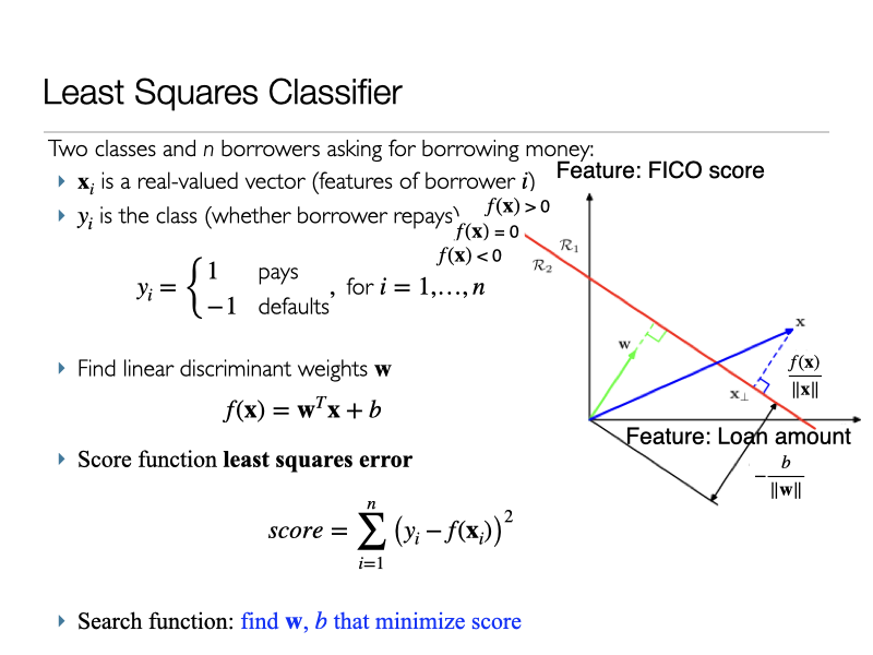
- Given ${\bf x}$ features of a borrower (income, loan request, FICO score,…)
- Classify whether a borrower will repay a loan based on their features ${\bf x}$
2. Quiz
With respect to ${\bf w}_1$, is the linear regression score $$\frac{1}{n} \sum_{i=1}^{n} \big(y_i - x_{i,1} {\bf w}_1 - x_{i,2} {\bf w}_2 - b \big)^2$$
- (a) Concave
- (b) Convex
- (c) Neither
- Hint 1: Collapse all terms that don't depend or multiply ${\bf w}_1$ into a single constant $c_i$: $\frac{1}{n} \sum_{i=1}^{n} \big(c_i - x_{i,1} {\bf w}_1 \big)^2$.
- Hint 2: Compute the second derivative of the above score with respect to ${\bf w}_1$.
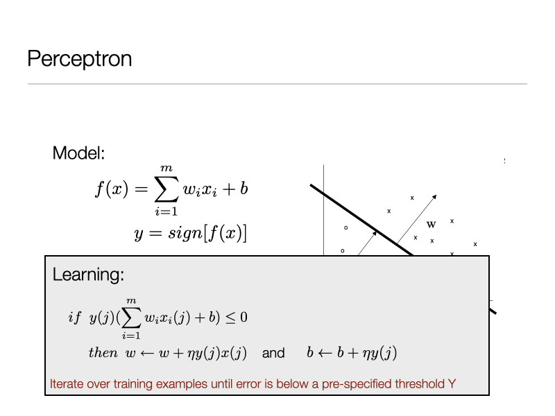
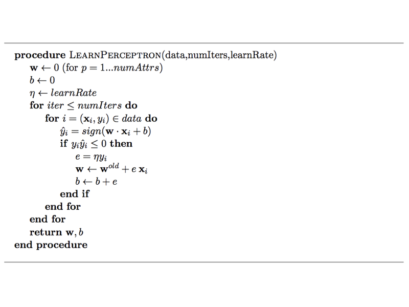
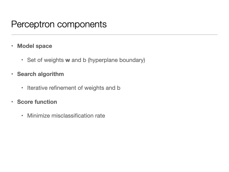
3. Perceptron algorithm

4. What about the Least Squares Regression for Classification?
Linear Regression for Classification
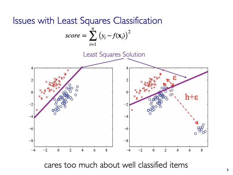
img credit: Bishop's book
5. Logistic Regression: Solving the Linear Regression issue for classification
5.1. Logistic Regression for Supervised Learning (Classification)
Consider the following task. We want to decide the probability that someone is rich. The input data is $\{(x_{i,1},x_{i,2}),y_i\}_i$ where input $x_{\cdot,1} \in {0,1}$ indicates yatch ownership, $x_{\cdot,2} \in {0,1}$ indicates mansion ownership, and $y_{\cdot} \in \{0,1\}$ indicates whether the person is rich. A logistic regression model can be represented as:
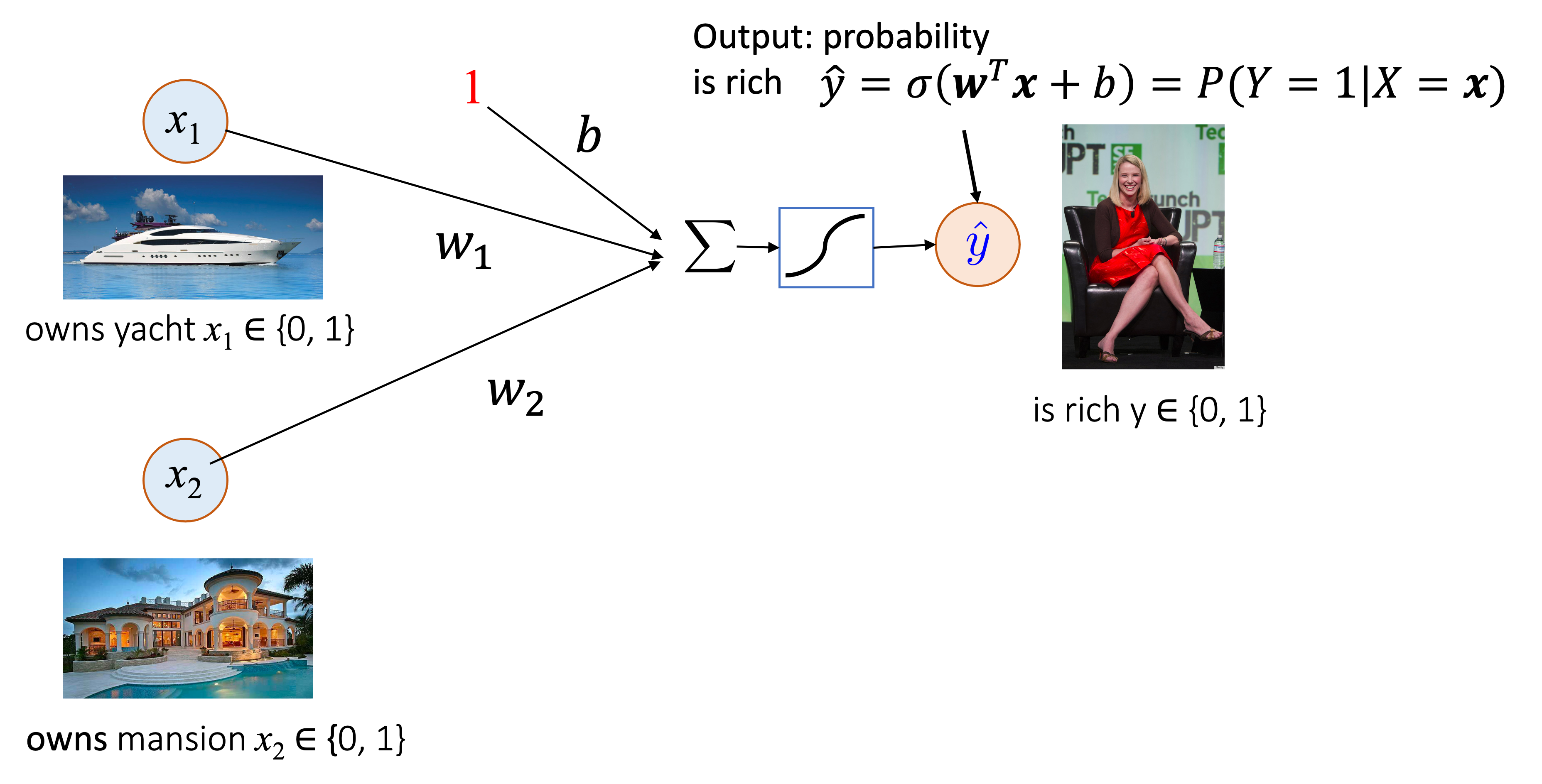
The s-shappped symbol after $\sum$ represents the sigmoid function.
5.2. Logistic Regression (LR) (for classification)
- Assume label $Y$ has two classes, $0$ and $1$
- Similar to predicting the probability of a Bernoulli "biased coin"
- Given $x$ what is the probability of $Y=1|X=x$?
5.3. Data Representation
Given an object's attribute vector ${\bf x} = (x_l, \ldots , x_p)$ with $p$ real-valued features, predict the object's class $y \in \{0,1\}$.
- Training data: $\{({\bf x}(1),y(1)),\ldots,({\bf x}(n),y(n))\}$
- Example: Let $p=2$ in the following example.
### Data Example
from sklearn.datasets import make_moons
from sklearn.model_selection import train_test_split
import pylab
import numpy as np

X, y = make_moons(n_samples=5000, random_state=42, noise=0.1)
X_train, X_test, y_train, y_test = train_test_split(X, y, random_state=42,test_size=0.3)

pylab.scatter(X[:,0], X[:,1], c=y)
pylab.xlabel("$x_1$",size=22)
pylab.ylabel("$x_2$",size=22)
pylab.show()

5.4. Knowledge Representation
We will consider a Logistic Regression model.
- Logistic regression model: $$ f({\bf x}) = {\bf w}^T {\bf x} + b = \sum_{j=1}^p w_j x_j + b,$$ with $$ P(y = 1 | {\bf x}; {\bf w}) = \sigma(f({\bf x})), $$ where $\sigma(a) = \frac{\exp(a)}{1+\exp(a)}$ is the sigmoid function.
- Alternative model
- Let ${\bf x}' = (1,{\bf x})$
- Let ${\bf w} = (b,w_1,\ldots,w_p)$.
- Logistic regression model: $$ P(Y=1| X={\bf x}) = \sigma( f({\bf x'})) = \sigma({\bf w}^T {\bf x}'), $$ with $\sigma$ again as the sigmoid function $$ \sigma(a) = \frac{\exp(a)}{1+\exp(a)}. $$
### Plot sigmoid function

import numpy as np
import matplotlib.pyplot as plt

# Sigmoid function
#
def sigmoid(a):
    return 1 / (1 + np.exp(-a))
# Creating sample f points
#
f = np.arange(-5, 5, 0.1)

# Invoking Sigmoid function on all Z points
#
sigma_f = sigmoid(f)

# Plotting the Sigmoid function
#
plt.plot(f, sigma_f)
plt.axvline(0.0, color='k')
plt.xlabel('$f(x)$',size=24)
plt.ylabel('$\sigma(f(x))$',size=24)
plt.yticks([0.0, 0.5, 1.0],size=24)
plt.xticks([-4, -2, 0 , 2, 4],size=24)
ax = plt.gca()
ax.yaxis.grid(True)
plt.tight_layout()
plt.show()

5.5. Decision boundary between classes (we will revisit this later)
- The logistic uses the inner product between ${\bf w}$ and ${\bf x}$: It gives the length of projection of ${\bf x}$ onto ${\bf w}$.
- If inner product is 0, then if ${\bf x}$ is perpendicular to ${\bf w}$
- Note that $\sigma(0) = 0.5$, which means $P(Y=1| X={\bf x}) = \sigma(0) = 0.5$
- Decision boundary is therefore linear (and divides the space into the two classes). The decision boundary is:
- a point if $p=1$
- a line if $p=2$
- a plane if $p = 3$
- a hyperplane if $p \geq 4$
- Now add b,
- if $f({\bf x}) > 0$, then $\sigma(f({\bf x})) > 0.5$
- if $f({\bf x}) < 0$, then $\sigma(f({\bf x})) < 0.5$
import numpy as np
import pylab

# We initialize weights and bias here with arbitrary values for a decision boundary.
w = np.array([1, -1])  # Weight vector w
b = 0.5  # Bias term
x1_vals = np.linspace(-1.5, 2.5, 100)  # x1 values range from -1.5 to 2.5
x2_vals = -(w[0] * x1_vals + b) / w[1]  # Compute x2 values using the decision boundary equation

# Scatter plot of the data points with class labels.
pylab.scatter(X[:, 0], X[:, 1], c=y)  # Plot data points with color indicating class (y)

# Plot the decision boundary line (x2 vs x1 based on the linear equation).
pylab.plot(x1_vals, x2_vals, label="Decision Boundary", color='red')

# Add the weight vector (w) as an arrow starting from the origin (0, 0).
origin = np.array([0, 0])  # Define origin at (0, 0)
pylab.quiver(*origin, *w, scale=5, color='purple')  # Draw an arrow representing vector w

# Add a text label "w" near the arrow to identify the weight vector.
pylab.text(w[0] - 0.5, w[1], 'w', color='purple', fontsize=15, ha='center', va='center')  # Label the vector

# Add vertical and horizontal black lines to mark the axes (thin lines).
pylab.axhline(y=0, color='black', linewidth=0.5)  # Draw horizontal x-axis at y=0
pylab.axvline(x=0, color='black', linewidth=0.5)  # Draw vertical y-axis at x=0

# Set y-axis limit so that it extends to -1.5.
pylab.ylim(-1.5, None)  # Set the lower limit of the y-axis to -1.5, leaving the upper limit unchanged

# Define and plot specific points relative to the decision boundary.
point_on_boundary = np.array([0, -b / w[1]])  # A point exactly on the decision boundary
point_near_boundary = np.array([0, (-b / w[1]) + 0.5])  # A point slightly above the decision boundary
point_far_from_boundary = np.array([1, -1])  # A point farther away from the decision boundary

# Scatter plot these specific points with distinct colors for visualization.
pylab.scatter(point_on_boundary[0], point_on_boundary[1], color='green', label='On boundary', s=100)
pylab.scatter(point_near_boundary[0], point_near_boundary[1], color='lightblue', label='Near boundary', s=100)
pylab.scatter(point_far_from_boundary[0], point_far_from_boundary[1], color='orange', label='Far from boundary', s=100)

# Set labels for x and y axes.
pylab.xlabel("$x_1$", size=22)  # Label for x-axis (x1)
pylab.ylabel("$x_2$", size=22)  # Label for y-axis (x2)

# Add a legend to explain the plotted points and decision boundary.
pylab.legend()

# Display the plot.
pylab.show()

# Define the sigmoid function for probability calculation based on raw output z.
def sigmoid(z):
    return 1 / (1 + np.exp(-z))  # Sigmoid activation function

# Loop through each specific point to calculate its raw model output (z) and the probability of being in class 1.
for point in [point_on_boundary, point_near_boundary, point_far_from_boundary]:
    z = np.dot(w, point) + b  # Calculate the linear combination of inputs and weights (z = w · x + b)
    prob = sigmoid(z)  # Apply sigmoid to get the probability
    print(f"Point {point}:")
    print(f"    z = {z:.4f} (this is the raw model output before applying sigmoid)")
    print(f"    Probability of being in class 1: {prob:.4f}\n")  # Display the probability for class 1

Point [0.  0.5]:
    z = 0.0000 (this is the raw model output before applying sigmoid)
    Probability of being in class 1: 0.5000

Point [0. 1.]:
    z = -0.5000 (this is the raw model output before applying sigmoid)
    Probability of being in class 1: 0.3775

Point [ 1 -1]:
    z = 2.5000 (this is the raw model output before applying sigmoid)
    Probability of being in class 1: 0.9241
5.6. Logistic Regression Graphical Depiction

6. Hands-on Example
6.1. Data & Knowledge representation for two moons example
The training data:
- Training data: $\{({\bf x}(1),y(1)),\ldots,({\bf x}(n),y(n))\}$
- ${\bf x} = (x_{1},x_{2}) \in \mathbb{R}^2$ is the 2-dimensional input
- ${\bf w} = (w_1,w_2) \in \mathbb{R}^2$ are the logistic regression weights
- $b$ is the bias
- Note that we have added an extra dimension to ${\bf x}$ with constant value 1.
- This is because sometimes it is easier to define $b = w_0$
6.2. Model space
- The model space of logistic regression is ${\bf w} \in \mathbb{R}^p$ and $b \in \mathbb{R}$.
- For the two moons example, $p=2$.
6.3. (Recap) Likelihood of Bernoulli Trials
Before we calculte the score function of logistic regression, recall that if $Y(1), \ldots, Y(n)$ are independent Bernoulli trials with parameters $p_1, \ldots, p_n$. The probability for each trial is defined as:
$$ P(Y(i) = 1 | p_i) = p_i \quad \text{and} \quad P(Y(i) = 0 | p_i) = 1 - p_i. $$
Since the trials are independent, the joint probability (likelihood) of observing outcomes $Y(1) = y(1), \ldots, Y(n) = y(n)$ is:
$$ P(Y(1) = y(1), \ldots, Y(n) = y(n) | p_1, \ldots, p_n) = \prod_{i=1}^n p_i^{y(i)} (1 - p_i)^{1 - y(i)}. $$
6.4. Negative Log-Likelihood of Observations
To simplify computations, we often work with the log-likelihood, which is the logarithm of the joint probability:
$$ \log P(Y(1) = y(1), \ldots, Y(n) = y(n) | p_1, \ldots, p_n) = \log \prod_{i=1}^n p_i^{y(i)} (1 - p_i)^{1 - y(i)}. $$
Using the property of logarithms that $\log(ab) = \log(a) + \log(b)$, we can split the log of a product into a sum of logs:
$$ = \sum_{i=1}^n \log \left( p_i^{y(i)} (1 - p_i)^{1 - y(i)} \right). $$
Next, apply the logarithm rule $\log(a^b) = b \log(a)$ to both terms inside the sum:
$$ = \sum_{i=1}^n \left( y(i) \log p_i + (1 - y(i)) \log (1 - p_i) \right). $$
Thus, the negative log-likelihood (NLL), which is also our score function, is:
$$ -\log P(Y(1) = y(1), \ldots, Y(n) = y(n) | p_1, \ldots, p_n) = - \sum_{i=1}^n \left( y(i) \log p_i + (1 - y(i)) \log (1 - p_i) \right). $$
6.5. Applying the Logistic Model
In logistic regression, the probability $p_i$ is modeled as:
$$ p_i = \sigma(\mathbf{w}^T \mathbf{x}(i) + b), $$
where $\sigma(z) = \frac{1}{1 + e^{-z}}$ is the sigmoid function. Substituting $p_i$ into the negative log-likelihood, the score function becomes:
$$ - \sum_{i=1}^n \left( y(i) \log \sigma(\mathbf{w}^T \mathbf{x}(i) + b) + (1 - y(i)) \log (1 - \sigma(\mathbf{w}^T \mathbf{x}(i) + b)) \right). $$
This is the final score function for logistic regression.
6.6. Model search
- To find the best model, we minimize the score (negative log-likelihood) over parameters ${\bf w}$ and $b$
- The above score is also described as cross-entropy loss, logistic loss, log loss, on Tensorflow, Sklearns, and PyTorch.
Gradient descent to find optimal values ${\bf w}^\star, b^\star$: $$\begin{align*} {\bf w}^\star, b^\star &={\arg\!\min}_{{\bf w},b} - \frac{1}{n} \sum_{i=1}^n \log P(Y = y(i) | X={\bf x}(i); {\bf w},b ) \\ &= {\arg\!\min}_{{\bf w},b} - \frac{1}{n} \sum_{i=1}^n y(i) \log \sigma({\bf w}^T {\bf x}(i) + b) + (1-y(i)) \log (1-\sigma({\bf w}^T {\bf x}(i) + b)) , \end{align*} $$ where $\sigma(x) = \frac{\exp(x)}{1 + \exp(x)}$.
6.7. Logistic Regression Convexity
- The negative log-likelihood of the logistic regression is convex in ${\bf w}$.
- That is, the NLL has a “bowl-shaped” graph.
- This means gradient descent should always go in the direction of the minimum loss until it is zero.
Start of code example
# There are only two features in the data X[:,0] and X[:,1]
n_features = 2
# There are only two classes: 0 (purple points) and 1 (yellow points)
n_class = 2

def init_weights(n_features):
    # Initialize weights with Standard Normal random variables
    model = dict(
        w=np.random.randn(n_features + 1, 1),
    )
    return model

model = init_weights(n_features=n_features)

print(model)
{'w': array([[-0.00129096],
       [ 1.04820381],
       [-0.26972077]])}
6.8. Model Search: Minimizing score function by gradient descent
Obtaining ${\bf w}$ via gradient descent:
- What are the derivatives?
- $\frac{\partial}{\partial w_1} \log \sigma({\bf w}^T {\bf x}(i) + b)$
- $\frac{\partial}{\partial w_2} \log \sigma({\bf w}^T {\bf x}(i) + b)$
- $\frac{\partial}{\partial b} \log \sigma({\bf w}^T {\bf x}(i) + b)$
- $\frac{\partial}{\partial w_1} \log (1-\sigma({\bf w}^T {\bf x}(i) + b))$
- $\frac{\partial}{\partial w_2} \log (1-\sigma({\bf w}^T {\bf x}(i) + b))$
- $\frac{\partial}{\partial b} \log (1-\sigma({\bf w}^T {\bf x}(i) + b))$
6.8.1. Gradient Facts
- Fact 1: $\frac{\partial}{\partial a} \log(a) = \frac{1}{a}$.
- Fact 2: For any function $g$, $\frac {\partial}{\partial a}\log g(a)=\frac {1}{g(a)}{\frac {\partial g(a)}{\partial a}}$
- Fact 3: $\frac{\partial}{\partial a} \sigma(a) = \sigma(a)(1-\sigma(a))$, where $\sigma$ is the sigmoid function.
- Fact 4 (chain rule): For continuous differentiable functions $f$ and $g$, $\frac{\partial}{\partial a} f(g(a)) =\left(\frac{\partial}{\partial b}f(b)\big|_{b = g(a)}\right)\frac{\partial}{\partial a}g(a)$
6.8.2. Finding the gradients
- Combining all the above facts we obtain our first derivative:
$$\begin{align*} & \frac{\partial}{\partial w_1} y(i) \log \sigma(w_1 {\bf x}_1(i) + w_2 {\bf x}_2(i) + b)\\ & = y(i) \frac{1}{\sigma({\bf w}^T {\bf x}(i) + b)} \frac{\partial}{\partial w_1} \sigma(w_1 {\bf x}_1(i) + w_2 {\bf x}_2(i) + b) \tag{from fact 2} \\ &= y(i) \frac{1}{\sigma({\bf w}^T {\bf x}(i) + b)} \big(\frac{\partial}{\partial a} \sigma(a)\big|_{a = {\bf w}^T {\bf x}(i) + b}\big) {\bf x}_1(i) \tag{from fact 4} \\ &= y(i) \frac{1}{\sigma({\bf w}^T {\bf x}(i) + b)} \sigma({\bf w}^T {\bf x}(i) + b) (1-\sigma({\bf w}^T {\bf x}(i) + b)) {\bf x}_1(i) \tag{from fact 3} \\ &= y(i) (1-\sigma({\bf w}^T {\bf x}(i) + b)) {\bf x}_1(i) \end{align*}$$
We can follow similar steps to obtain all other derivatives:
- $\frac{\partial}{\partial w_2} y(i) \log \sigma(w_1 {\bf x}_1(i) + w_2 {\bf x}_2(i) + b) = y(i) (1-\sigma({\bf w}^T {\bf x}(i) + b)) {\bf x}_2(i)$
- $\frac{\partial}{\partial b} y(i) \log \sigma(w_1 {\bf x}_1(i) + w_2 {\bf x}_2(i) + b) = y(i) (1-\sigma({\bf w}^T {\bf x}(i) + b))$
- $\frac{\partial}{\partial w_1} (1- y(i)) \log (1-\sigma(w_1 {\bf x}_1(i) + w_2 {\bf x}_2(i) + b)) = -(1-y(i)) \sigma({\bf w}^T {\bf x}(i) + b) {\bf x}_1(i)$
- $\frac{\partial}{\partial w_2} (1- y(i)) \log (1-\sigma(w_1 {\bf x}_1(i) + w_2 {\bf x}_2(i) + b)) = -(1-y(i)) \sigma({\bf w}^T {\bf x}(i) + b) {\bf x}_2(i)$
- $\frac{\partial}{\partial b} (1- y(i)) \log (1-\sigma(w_1 {\bf x}_1(i) + w_2 {\bf x}_2(i) + b)) = -(1-y(i)) \sigma({\bf w}^T {\bf x}(i) + b)$
Note that
- $\frac{\partial}{\partial w_1} y(i) \log \sigma(w_1 {\bf x}_1(i) + w_2 {\bf x}_2(i) + b) +\frac{\partial}{\partial w_1} (1- y(i)) \log (1-\sigma(w_1 {\bf x}_1(i) + w_2 {\bf x}_2(i) + b)) = (\sigma(w_1 {\bf x}_1(i) + w_2 {\bf x}_2(i) + b) - y(i)) {\bf x}_1(i)$
- We will call $(\sigma(w_1 {\bf x}_1(i) + w_2 {\bf x}_2(i) + b) - y(i))$ the error.
# Defines sigmoid function
def sigmoid(a):
    return (1 / (1 + np.exp(-a)))

# For a single example $x$
def logistic_regression(x, model):
    x = np.append(x, 1)

    # Input times weight vector
    f_x = x @ model['w']

    # Sigmoid activation
    y_hat = sigmoid(f_x)

    return y_hat
def logistic_derivative(model, xs, errors):
    """xs, errs contain all information (input, error) of all the data"""
    # gradient of the negative log-likelihood with respect to model parameters
    dw = xs.T @ errors

    return dict(w=dw)
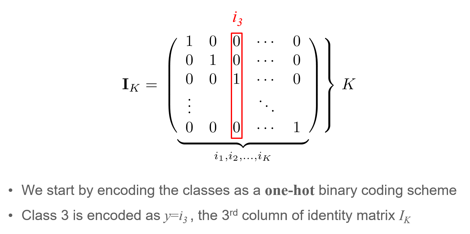
One-hot encoding: Encoding of the target variable $y$ for $K$ classes ($K=2$ in our case)
# Get gradient of all parameters

def get_gradient(model, X_train, y_train):
    xs, errors = [], []

    for x, cls_idx in zip(X_train, y_train):
        y_pred = logistic_regression(x, model)

        # Create one-hot coding of true label
        y_true = np.zeros(n_class)
        y_true[int(cls_idx)] = 1.

        error = y_pred - y_true[1]

        # Accumulate the informations of the examples
        # x: all inputs
        # error: all errors
        x = np.append(x, 1)
        xs.append(x)
        errors.append(error)

    # Get gradients
    return logistic_derivative(model, np.array(xs), np.array(errors))
6.8.3. Define one gradient descent step
We now perform a single gradient descent step.
Update ${\bf w}_1$: Get the gradients and perform the following updates for $N$ training examples: $$ {\bf w}_1 ={\bf w}_1 - \epsilon \sum_{i=1}^n \frac{\partial \text{Score}(i)}{\partial {\bf w}_1}, $$ where $\frac{\partial \text{Score}(i)}{\partial {\bf w}_1} = (\sigma(w_1 {\bf x}_1(i) + w_2 {\bf x}_2(i) + b) - y(i)) {\bf x}_1(i)$ and $\epsilon$ is our learning rate.
Update ${\bf w}_2$: $${\bf w}_2 ={\bf w}_2 - \epsilon \sum_{i=1}^n \frac{\partial \text{Score}(i)}{\partial {\bf w}_2},$$ where $\frac{\partial \text{Score}(i)}{\partial {\bf w}_2} = (\sigma(w_1 {\bf x}_1(i) + w_2 {\bf x}_2(i) + b) - y(i)) {\bf x}_2(i)$.
Update $b$:$$b =b - \epsilon \sum_{i=1}^n \frac{\partial \text{Score}(i)}{\partial b},$$ where $\frac{\partial \text{Score}(i)}{\partial b} = (\sigma(w_1 {\bf x}_1(i) + w_2 {\bf x}_2(i) + b) - y(i))$
def one_gradient_step(model, X_train, y_train, learning_rate=1e-2):
    grad = get_gradient(model, X_train, y_train)

    # Update all parameters in the parameter dictionary
    for param in grad:
        # Learning rate: default 1e-2
        model[param] -= learning_rate * grad[param]

    return model
def gradient_descent(model, X_train, y_train, no_iter=10):
    for epoch in range(no_iter):

        if epoch % 10 == 0:
            print(f'Epoch {epoch}')

        model = one_gradient_step(model, X_train, y_train)

    print(f'Epoch {epoch}')
    return model
no_iter = 100

# Reset model
model = init_weights(n_features)

# Search for best parameters to minimize score function
model = gradient_descent(model, X_train, y_train, no_iter=no_iter)
Epoch 0
Epoch 10
Epoch 20
Epoch 30
Epoch 40
Epoch 50
Epoch 60
Epoch 70
Epoch 80
Epoch 90
Epoch 99
6.9. Test learned model
Now we will a separate held out dataset (test data) in order to test the accuracy of our model.
y_pred = np.zeros_like(y_test)

accuracy = 0

for i, x in enumerate(X_test):
    # Predict the distribution of label
    y_hat = logistic_regression(x, model)
    # Get label by picking the most probable class
    y = (y_hat[0] > 0.5).astype(int)
    y_pred[i] = y

# Accuracy of predictions with the true labels and take the percentage
# Because our dataset is balanced, measuring just the accuracy is OK
accuracy = (y_pred == y_test).sum() / y_test.size
print('Test accuracy after {} gradient steps: {}'.format(no_iter,accuracy))

pylab.scatter(X_test[:,0], X_test[:,1], c=y_pred)
pylab.show()
Test accuracy after 100 gradient steps: 0.8553333333333333

6.10. [IMPORTANT] Always add L1 or L2 regularization to logistic regression in case training data is linearly separable
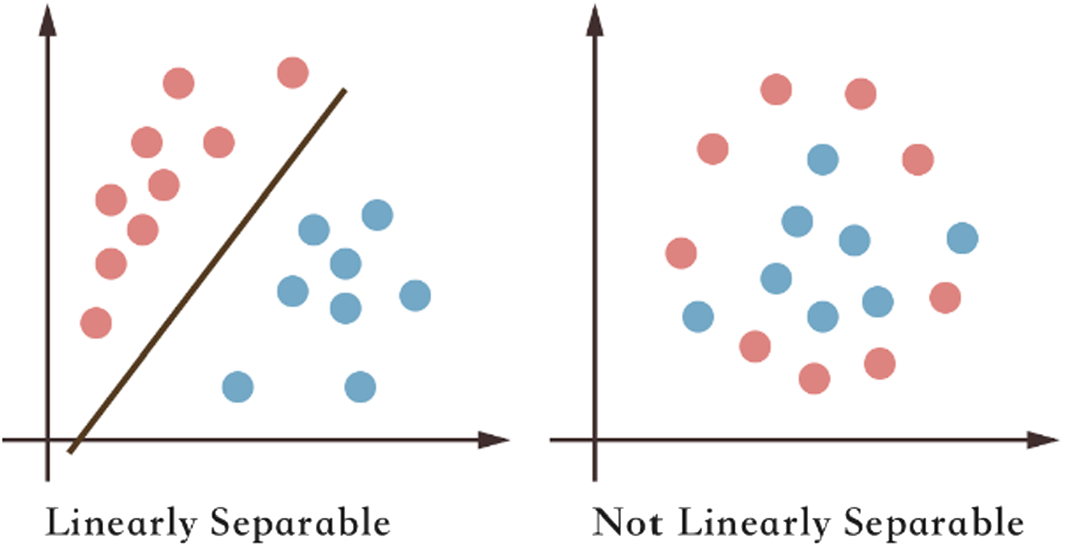
- For linearly separable data, as in the left figure in the image above, the classifier will want to set $\sigma({\bf w}^T {\bf x}(i) + b)$ such that the output of the sigmoid is either zero or one.
- This means gradient descent keep trying to increase $\Vert {\bf w} \Vert_1$, and it can always decrease the loss (score).
- Hence, it is important to add L1 or L2 regularization to the standard negative log-likelihood loss (score).
- With regularization, continuously increasing (or decreasing) the values in ${\bf w}$ eventually stops because of the added loss $\Vert {\bf w} \Vert_1$ of our L1 regularization.
7. (Extra) What about multiple classes?
- We have seen that using multiple binary classifiers is not ideal
- How should we deal with multiple classes?

7. Multiclass Logistic Regression
7.1. Logistic Regression for multiple classes
- Consider $K$ classes and $n$ observations
- Let $y_i$ be the class of the $i$-th example with feature vector $x_i$.
- The probability that $x_i$ belongs to class $k$ is: $$ P(Y=k|X = x_i) = \frac{\exp({\bf w}_k^T x_i)}{\sum_{k' = 1}^K \exp({\bf w}_{k'}^T x_i)} ,\quad k=1,\ldots,K. $$
- The new model space is a matrix ${\bf W} \in \mathbb{R}^{K \times p+1}$.
- A matrix version of the above calculation gives
$$
\left[ \begin{array}{cccc}
P(Y=1|x_i) \\
P(Y=2|x_i)\\
\vdots \\
P(Y=K|x_i)
\end{array} \right]
= \text{softmax}\left(
\left[ \begin{array}{cccc}
W_{11} & W_{12} & \ldots & W_{1p} \\
W_{21} & W_{22} & \ldots & W_{2p} \\
\vdots &\vdots & \ldots & \vdots \\
W_{K1} & W_{K2} & \ldots & W_{Kp} \\
\end{array} \right]
\cdot
\left[ \begin{array}{cccc}
x_1 \\
x_2\\
\vdots \\
x_p
\end{array} \right] \right),
$$
where
sotfmax$({\bf b})$ is the application of $\frac{\exp({\bf b}_j)}{\sum_{j'} \exp({\bf b}_{j'})}$ over each element of a vector ${\bf b}$.
7.2. Logistic Regression for multiple classes (Step 1): Encoding of the output $y$
7.3. Logistic Regression for multiple classes (Step 2): Log-likelihood
Assume $y(i)$ is one-hot encoded as described above of the $i$-th training example, and ${\bf x}(i)$ is its feature input.
The output of $f$ is a vector of $K$ probabilities.
Then, $$\text{Score} = \sum_{i=1}^n \text{Score}(i) = -\sum_{i=1}^n \sum_{j=1}^K y_{j}(i) \log \sigma(f({\bf x}(i);{\bf W})_j), $$ where $(z)_j$ is the $j$-th element of $z$'s vector.
7.3.1. Example of Multiclass Logistic Regression for $K=2$
# There are only two features in the data X[:,0] and X[:,1]
n_features = 2
# There are only two classes: 0 (purple points) and 1 (yellow points)
n_class = 2

def multiclass_init_weights(n_features):
    # Initialize weights with Standard Normal random variables
    model = dict(
        W=np.random.randn(n_features + 1, n_class),
    )
    return model

model = multiclass_init_weights(n_features=n_features)

print(model)
{'W': array([[ 1.25320278, -0.67771525],
       [ 0.38927771,  0.86286996],
       [-0.23545144, -1.19446593]])}
# Defines the softmax function.
def softmax(x):
    return np.exp(x) / np.exp(x).sum()


# For a single example $x$
def multiclass_logistic_regression(x, model):
    x = np.append(x, 1)

    # Input times weight vector
    f_x = x @ model['W']

    # Softmax activation
    y_hat = softmax(f_x)

    return y_hat
def multiclass_logistic_derivative(model, xs, errors):
    """xs, errs contain all information (input, error) of all the data"""
    # gradient of the negative log-likelihood with respect to model parameters
    dW = xs.T @ errors

    return dict(W=dW)
# Get gradient of all parameters

def multiclass_get_gradient(model, X_train, y_train):
    xs, errors = [], []

    for x, cls_idx in zip(X_train, y_train):
        y_pred = multiclass_logistic_regression(x, model)

        # Create one-hot coding of true label
        y_true = np.zeros(n_class)
        y_true[int(cls_idx)] = 1.

        error = y_pred - y_true

        # Accumulate the informations of the examples
        # x: all inputs
        # error: all errors
        x = np.append(x, 1)
        xs.append(x)
        errors.append(error)

    # Get gradients
    return multiclass_logistic_derivative(model, np.array(xs), np.array(errors))
def multiclass_one_gradient_step(model, X_train, y_train, learning_rate=1e-2):
    grad = multiclass_get_gradient(model, X_train, y_train)

    # Update all parameters in the parameter dictionary
    for param in grad:
        # Learning rate: default 1e-2
        model[param] -= learning_rate * grad[param]

    return model
def multiclass_gradient_descent(model, X_train, y_train, no_iter=10):
    for epoch in range(no_iter):

        if epoch % 10 == 0:
            print(f'Epoch {epoch}')

        model = multiclass_one_gradient_step(model, X_train, y_train)

    print(f'Epoch {epoch}')
    return model
no_iter = 100

# Reset model
model = multiclass_init_weights(n_features)

# Train the model
model = multiclass_gradient_descent(model, X_train, y_train, no_iter=no_iter)
Epoch 0
Epoch 10
Epoch 20
Epoch 30
Epoch 40
Epoch 50
Epoch 60
Epoch 70
Epoch 80
Epoch 90
Epoch 99
y_pred = np.zeros_like(y_test)

accuracy = 0

for i, x in enumerate(X_test):
    # Predict the distribution of label
    y_hat = multiclass_logistic_regression(x, model)
    # Get label by picking the most probable one
    y = np.argmax(y_hat)
    y_pred[i] = y

# Accuracy of predictions with the true labels and take the percentage
# Because our dataset is balanced, measuring just the accuracy is OK
accuracy = (y_pred == y_test).sum() / y_test.size
print('Test accuracy after {} gradient steps: {}'.format(no_iter,accuracy))

pylab.scatter(X_test[:,0], X_test[:,1], c=y_pred)
pylab.show()
Test accuracy after 100 gradient steps: 0.8486666666666667

Step 1: Understanding Pytorch's Automatic Differentiation
First, we will create a variable $x \in \mathbb{R}$ and assign it value $x = 3$.
### The following code is intuitive but **WRONG**

import torch

x = torch.zeros(1, requires_grad=True) # Assigns a constant zero to unidimensional variable x
                                       # requires_grad=True tells pytorch we will compute gradients for this variable

x = 3. ## Here we assign float(3.) to "x" ... which is no longer a differentiable torch tensor

print(f'Value of x = {x.data}') # Will return an error because now x is a float value
print(f'Gradient of x = {x.grad}') # Will return None because it we need to invoke .backward() first
---------------------------------------------------------------------------
AttributeError                            Traceback (most recent call last)
Cell In[20], line 10
      6                                        # requires_grad=True tells pytorch we will compute gradients for this variable
      8 x = 3. ## Here we assign float(3.) to "x" ... which is no longer a differentiable torch tensor
---> 10 print(f'Value of x = {x.data}') # Will return an error because now x is a float value
     11 print(f'Gradient of x = {x.grad}') # Will return None because it we need to invoke .backward() first

AttributeError: 'float' object has no attribute 'data'
- This is the correct way to attribute values to differentiable variables in pyTorch
import torch

x = torch.zeros(1, requires_grad=True) # Assigns a constant zero to unidimensional variable x
                                       # requires_grad=True tells pytorch we will compute gradients for this variable
x.data.fill_(3.)

print(f'Value of x = {x.data}') # Will return 1 as a tersor variable
print(f'Gradient of x = {x.grad}') # Will return None because it we need to invoke .backward() first
Value of x = tensor([3.])
Gradient of x = None
Consider the following function: $$ z(x) = 10 y(x)^2, $$ where $$ y(x) = 2 x + 1. $$
Now, let's compute $$\left. \frac{\partial z(x)}{\partial x} \right|_{x = 3}.$$
x = torch.zeros(1, requires_grad=True) # Assigns a constant zero to unidimensional variable x
                                       # requires_grad=True tells pytorch we will compute gradients for this variable

x.data.fill_(3.) # Constant MUST be floating point (if the tensor is an Integer, it won't work)

y = 2 * x + 1
z = 10 * y * y
z.backward()     # automatically computes the gradient ∂z/∂x evaluated at x = 1 using backpropagation
print(x.grad)    # ∂z/∂x = 280
tensor([280.])
Step 2: Create Logistic Regression Model using Pytorch Libraries
import torch.nn as nn
import torch.nn.functional as F

class LogisticRegression(nn.Module):
    def __init__(self, input_size, output_size): ## This will also take care of initilizing the weights
        super(LogisticRegression, self).__init__()
        self.f_x = nn.Linear(input_size, output_size)
        self.output_size = output_size

    def forward(self, x):
        if self.output_size == 1:
            y_hat = torch.sigmoid(self.f_x(x))
        else:
            y_hat = F.softmax(self.f_x(x),dim=0)  # dim is the dimension along the softmax will be computed
        return y_hat
Can we use a GPU?
use_cuda = torch.cuda.is_available()  # Our flag to check if Nvidia GPU is available

device = torch.device("cuda" if use_cuda else "cpu") # Decide device between CUDA (GPU) and CPU compute

print(f'Is CUDA available? {use_cuda}')
Is CUDA available? False
Move training data into Torch tensors
- Training data becomes a tensor
- One of the tensor dimensions is the number of training examples
- The data moves to the GPU if device = torch.device("cuda")
# Transform original data into pytorch tensors and send to device (send data to GPU if available)
torch_X_train = torch.FloatTensor(X_train).to(device)
torch_X_test = torch.FloatTensor(X_test).to(device)
torch_y_train = torch.FloatTensor(y_train).to(device)
torch_y_test = torch.FloatTensor(y_test).to(device)

print(f'Now data is in Pytorch tensor form: {torch_y_train}')
Now data is in Pytorch tensor form: tensor([1., 0., 0., ..., 1., 0., 1.])
Instantiate logistic regression
Creates a Logistic Regression model with
- 2-dimensional input
- 1-dimensional
sigmoidoutput - Default weight initialization
- Linear layer weight and bias values are initialized by sampling $\text{Uniform}(-\sqrt{k}, \sqrt{k})$, where $k = \frac{1}{\text{in_dimension}}$
##    Send model parameters to "device" (GPU if the device is on the GPU)
LR = LogisticRegression(input_size = 2, output_size = 1).to(device)

print(f'Logistic regression model created: {LR}')
Logistic regression model created: LogisticRegression(
  (f_x): Linear(in_features=2, out_features=1, bias=True)
)
Logistic Regression prediction
Get current predicted training label probabilities from the logistic
y_pred = LR(torch_X_train) ### Get output of FeedForward network over the training data

print(f'Predicted values of X: {y_pred}')
Predicted values of X: tensor([[0.5371],
        [0.6012],
        [0.6617],
        ...,
        [0.5381],
        [0.6722],
        [0.6029]], grad_fn=<SigmoidBackward0>)
Compute the Negative log-likelihood score
- Define the loss function (negative log-likelihood score for unidimensional sigmoid outputs)
- Compute the loss
# Define the loss function
# Negative log-likelihood loss (aka, cross-entropy loss) for binary classes
loss = nn.BCELoss()

## Compute the loss of the predicted values
error = loss(y_pred, torch_y_train.view(-1,1)) ## .view(-1,1) avoids a warning about the tensor dimension
Use the loss to compute gradients
- Computes gradients from the loss via backpropagation
- Never forget to zero the gradient vectors first (Pytorch accumulate gradients by default)
# Compute the gradients of the logistic with respect to the error
##  Gradient computation performed via backpropagation

LR.zero_grad() ## Zero current gradients (Pytorch accumulate gradients by default)

error.backward() ## Compute gradients via backpropagation
Define the learning rate
- We will revisit the effect of learning rates later
- Very small learning rates can result in poor generalization error
- Commonly a number between 1 and 1e-05
## Define learning rate
learning_rate = 1e-2
Perform one gradient step
- Will subtract the (gradient * learning_rate) from all parameters
print(f"Before gradient step: Layer 1 bias {LR.f_x.bias}")

## Go over all parameters and subtract their gradient
##   Subtract (not sum) the gradient since we want to minimize the loss
for f in LR.parameters():
    f.data.sub_(f.grad.data * learning_rate)

print(f"After gradient step: Layer 1 bias {LR.f_x.bias}")
Before gradient step: Layer 1 bias Parameter containing:
tensor([0.1277], requires_grad=True)
After gradient step: Layer 1 bias Parameter containing:
tensor([0.1266], requires_grad=True)
Optimize the model
- We will now perform 1000 optimization steps using the entire dataset
- Epoch: Each time the entire dataset is used in the optimization
- It is useful to plot the training accuracy
## Loop through multiple gradient steps

for epoch in range(1000):
    ## Predict values using updated model
    y_pred = LR(torch_X_train)

    ## Find predicted class (as a number {1,0})
    pred = y_pred.gt(0.5) + 0.0

    # Compute accuracy
    if epoch % 100 == 9:
        correct = pred.eq(torch_y_train.view_as(pred)).sum().item()
        print(f'Epoch {epoch} training accuracy: {int(correct/torch_y_train.shape[0] * 100)}%')

    ## Compute the new error
    error = loss(y_pred, torch_y_train.view(-1,1)) ## .view(-1,1) avoids a warning about the tensor dimension

    LR.zero_grad() ## Zero current gradients (Pytorch accumulate gradients by default)

    error.backward() ## Compute gradients in Pytorch via backpropagation

    ## Go over all parameters and subtract their gradient
    for f in LR.parameters():
        f.data.sub_(f.grad.data * learning_rate)

## Final train accuracy
if epoch % 100 == 9:
    correct = pred.eq(torch_y_train.view_as(pred)).sum().item()
    print(f'Correct {int(correct/torch_y_train.shape[0] * 100)}%')
Epoch 9 training accuracy: 71%
Epoch 109 training accuracy: 73%
Epoch 209 training accuracy: 74%
Epoch 309 training accuracy: 76%
Epoch 409 training accuracy: 77%
Epoch 509 training accuracy: 78%
Epoch 609 training accuracy: 79%
Epoch 709 training accuracy: 79%
Epoch 809 training accuracy: 80%
Epoch 909 training accuracy: 80%
# Prepare model for evaluation (needed to avoid computing gradient)
with torch.no_grad():
    # Prepare model for evaluation (needed to avoid computing gradient)
    LR.eval()
    # Predict the distribution of label
    y_hat = LR(torch_X_test)
    # Get label by picking the most probable one
    y_pred = y_hat.gt(0.5) + 0.0

    # Accuracy of predictions with the true labels and take the percentage
    # Because our dataset is balanced, measuring just the accuracy is OK
    correct = y_pred.eq(torch_y_test.view_as(y_pred)).sum().item()
    print(f'Correctly classified test examples {int(correct/torch_y_test.shape[0] * 100)}%')

    pylab.scatter(X_test[:,0], X_test[:,1], c=y_pred)
    pylab.show()
Correctly classified test examples 82%

Extra: Weight initialization (we will revisit this when we talk about the optimization)
## Try different weight initializations of the linear layers
## Not needed, but you can apply a different initialization of the weights before optimizing

def init_weights(layer):
    if type(layer) == nn.Linear:
        torch.nn.init.normal_(layer.weight)
        layer.bias.data.fill_(0.01)

LR.apply(init_weights) ## Function apply will go over all layers
LogisticRegression(
  (f_x): Linear(in_features=2, out_features=1, bias=True)
)