Improved reweighted graphs
In MatlabBGL 3.0, reweighted graphs were a pain to use. Now they are simple! We combine a structural matrix with a weight matrix. As(i,j)=1 if there is an edge between vertex i and j and A(i,j)=wij where wij is the weight of the edge between i and j.
As = cycle_graph(6,'directed',0); % compute a 6 node cycle graph
A = As; % set all the weights to be one initially
A(2,3) = 0; A(3,2) = 0; % make one edge have zero weight
fprintf('Edges\n');
full(As)
fprintf('Weights\n');
full(A)
Edges

ans =

     0     1     0     0     0     1
     1     0     1     0     0     0
     0     1     0     1     0     0
     0     0     1     0     1     0
     0     0     0     1     0     1
     1     0     0     0     1     0

Weights

ans =

     0     1     0     0     0     1
     1     0     0     0     0     0
     0     0     0     1     0     0
     0     0     1     0     1     0
     0     0     0     1     0     1
     1     0     0     0     1     0
Note that As is given as the graph in the following call, not A!
[d pred] = shortest_paths(As,1,'edge_weight',edge_weight_vector(As,A));
d(3) % distance from vertex 1 to vertex 3 should be just 1!
ans =

     1
Graph layout algorithms
Sometimes, it's really nice to see a picture of your graph. The BGL implements a few graph layout algorithms and so these are now in MatlabBGL 4.0!
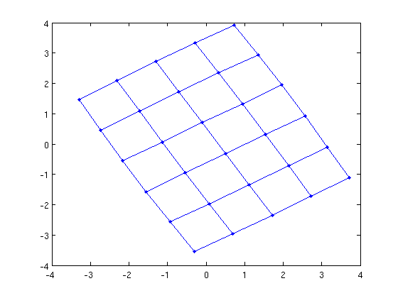
G = grid_graph(6,5);
X = kamada_kawai_spring_layout(G);
gplot(G,X,'.-');
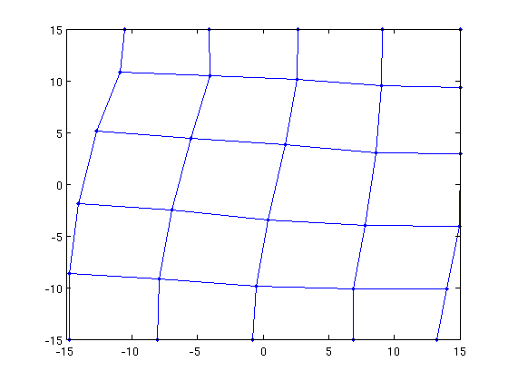
G = grid_graph(6,5);
X = fruchterman_reingold_force_directed_layout(G);
gplot(G,X,'.-');
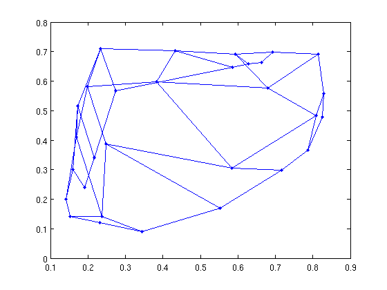
G = grid_graph(6,5);
X = gursoy_atun_layout(G);
gplot(G,X,'.-');
Planar graph algorithms
The Boost Graph Library received a new suite of planar graph algorithms. These are now in MatlabBGL too.
A grid in the xy plane is a planar graph.
G = grid_graph(6,5);
is_planar = boyer_myrvold_planarity_test(G)
is_planar =

     1
Recall that K_5 (the clique on 5 vertices) is not a planar graph. Let's see what happens.
K5 = clique_graph(5);
is_planar = test_planar_graph(K5) % helpful wrapper
is_planar =

     0
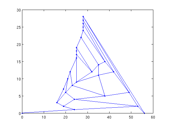
We can also draw planar graphs
G = grid_graph(6,5);
X = chrobak_payne_straight_line_drawing(G);
gplot(G,X,'.-'); % it looks a little different!
New option syntax
You probably noticed that the "struct" command that permeated MatlabBGL calls before is gone in these examples. We've moved to a new option syntax that gives you the choice between the MatlabBGL struct style arguments and a list of key-value pairs
We'll look at spanning trees on the clique graph with 5 vertices. Using Prim's algorithm, the spanning tree we get depends on the root. We always get a star graph rooted at the vertex we pick as the root.
G = clique_graph(5);
Old style
full(mst(G,struct('root',5,'algname','prim')))
ans =

     0     0     0     0     1
     0     0     0     0     1
     0     0     0     0     1
     0     0     0     0     1
     1     1     1     1     0
New style
Just to make sure it works
full(mst(G,'root',1,'algname','prim'))
ans =

     0     1     1     1     1
     1     0     0     0     0
     1     0     0     0     0
     1     0     0     0     0
     1     0     0     0     0