Better performance
We redid the backend interface to the BGL routines. This optimization gave a considerable performance increase.
test_benchmark on MatlabBGL 2.1
2008-10-07, Version 2.1, Matlab 2007b, boost 1.33.0,
  g++-3.4 (lib), gcc-? (mex)
       airfoil       west    cs-stan    minneso      tapir
large   0.223 s    0.024 s    0.390 s    0.073 s    0.046 s
  med     NaN s    0.955 s      NaN s      NaN s    6.621 s
small     NaN s    0.758 s      NaN s      NaN s      NaN s
test_benchmark on MatlabBGL 3.0
2008-10-07: Version 3.0, Matlab 2007b, boost 1.34.1,
  g++-4.0 (lib), gcc-? (mex)
       airfoil       west    cs-stan    minneso      tapir
large   0.183 s    0.017 s    0.222 s    0.048 s    0.037 s
  med     NaN s    0.593 s      NaN s      NaN s    3.901 s
small     NaN s    0.543 s      NaN s      NaN s      NaN s
Graph construction functions
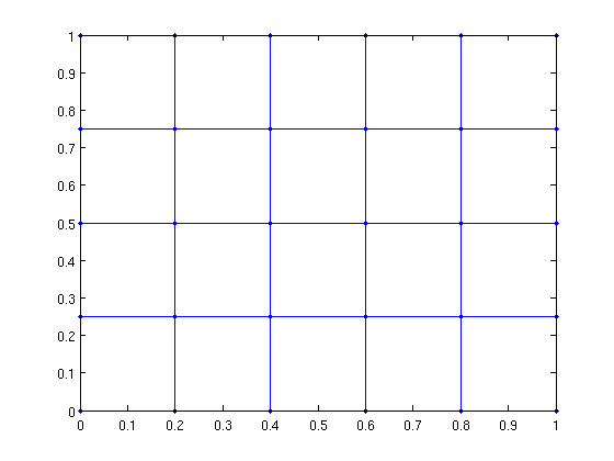
MatlabBGL 2.1 had a few graph construction functions. MatlabBGL 3.0 adds the grid_graph function for line, grid, cube, and hyper-cube graphs
[G xy] = grid_graph(6,5); gplot(G,xy,'.-');
In more dimensions...
[G xyz] = grid_graph(6,5,3);
G = grid_graph(2,2,2,2);
G = grid_graph([3,3,3,3,3]);
Targeted search
The graph search algorithms now let you specify a target vertex that will stop the search early if possible.
A = grid_graph(50,50);
tic; d = bfs(A,1,struct()); toc
tic; d = bfs(A,1,struct('target',2)); toc
Elapsed time is 0.001580 seconds.
Elapsed time is 0.000671 seconds.
Also implemented for astar_search, shortest_paths, and dfs.
Edge weights
In Matlab, there is no way to create a sparse matrix with a structural non-zero (used for MatlabBGL edges) and a value of 0 (used for MatlabBGL weights). Consequently, it's impossible to run algorithms on graphs where the edge weights are 0.
Consequently, some algorithms now take an 'edge_weight' parameter that allows you to provide a different set of edge weights which allow structural non-zeros and 0 values.
This behavior is a bit complicated, so see the REWEIGHTED_GRAPHS example for more information.
Matching algorithms
While maximum cardinality bipartite matching is just a call to max-flow, general graph matching algorithms are not. MatlabBGL 3.0 contains the matching algorithms in Boost 1.34.0.
load('../graphs/matching_example.mat');
m = matching(A);
sum(m>0)/2 % matching cardinality should be 8
ans =

     8
New graph statistics
We added a few new statistics functions.
Test for a topological ordering of a graph (only applies to DAGs or directed acyclic graphs)
n = 10; A = sparse(1:n-1, 2:n, 1, n, n); % construct a simple dag
p = topological_order(A);

test_dag(A)
test_dag(cycle_graph(6)) % a cycle is not acyclic!
ans =

     1


ans =

     0
Core numbers can help identify important regions in a graph. MatlabBGL includes weighted and directed core numbers. Also, the algorithms return the removal time of a particular vertex, which gives interesting graph orderings.
% See EXAMPLES/CORE_NUMBERS_EXAMPLE
New algorithms for clustering_coefficients on weighted and directed graphs.
A = clique_graph(6) - cycle_graph(6); % A is a clique - a directed cycle
ccfs = clustering_coefficients(A)
B = sprand(A);
ccfs = clustering_coefficients(B)
C = A|A'; % now it's a full clique again
ccfs = clustering_coefficients(C)
ccfs =

    0.7600
    0.7600
    0.7600
    0.7600
    0.7600
    0.7600


ccfs =

    0.3480
    0.4104
    0.4025
    0.4191
    0.4156
    0.4380


ccfs =

     1
     1
     1
     1
     1
     1
Max-flow algorithms
Since Boost added the Kolmogorov max-flow function, we added the full collection of flow algorithms to MatlabBGL.
load('../graphs/max_flow_example.mat');

push_relabel_max_flow(A,1,8)
kolmogorov_max_flow(A,1,8)
edmunds_karp_max_flow(A,1,8)

max_flow(A,1,8,struct('algname','push_relabel'));
max_flow(A,1,8,struct('algname','kolmogorov'));
max_flow(A,1,8,struct('algname','edmunds_karp'));
ans =

     4


ans =

     4


ans =

     4
Dominator tree
Dominator trees are relations about presidence in certain types of graphs. These are also called flow-graphs.
load('../graphs/dominator_tree_example.mat');
p = lengauer_tarjan_dominator_tree(A,1);
New utility functions
MatlabBGL 3.0 introduces some new utility functions.
The output of a shortest path algorithm is a predecessor matrix. To convert these predecessor relationships to a path, use the path_from_pred function.
[A xy] = grid_graph(6,5); n= size(A,1);
[d dt pred] = bfs(A,1); %
path = path_from_pred(pred,n) % sequence of vertices to upper corner
path =

     1     2     3     4     5     6    12    18    24    30
Let's draw the path
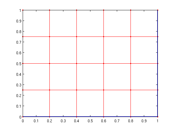
gplot(A,xy,'r.-');
[px,py]=gplot(sparse(path(1:end-1),path(2:end),1,n,n),xy,'-');
hold on; plot(px,py,'-','LineWidth',2); hold off;
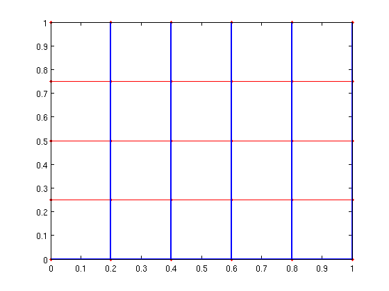
We can also create a full shortest path tree using the tree_from_pred function.
T = tree_from_pred(pred);
gplot(A,xy,'r.-');
[px,py]=gplot(T,xy,'-');
hold on; plot(px,py,'-','LineWidth',2); hold off;
Finally, there are a few new routines to make working with reweighted graphs easier. See EXAMPLES/REWEIGHTED_GRAPHS for information about the INDEXED_SPARSE and EDGE_WEIGHT_INDEX functions.