Giant Component
In this tutorial/record, we'll look at generating Erdos-Reyni random graphs in Matlab, and see the giant component in the graph.
The first step is to pick the number of vertices in the graph and the probability of an edge between two vertices.
>> n = 150;
>> p = 0.01;
With these two parameters, we can instantiate the graph.
The variable G is the adjacency matrix for the graph. The second operation symmetrizes the adjacency matrix
by discarding half of it.
>> G = rand(n,n) < p;
>> G = triu(G,1);
>> G = G + G';
From the theory of Erdos-Reyni graphs, we know that a giant connected component
should emerge when p > 1/(n-1).
>> thres_giant = 1/(n-1)
thres_giant =
0.0067
Because p = 0.01 > 0.0067, we expect our graph to have such a giant component.
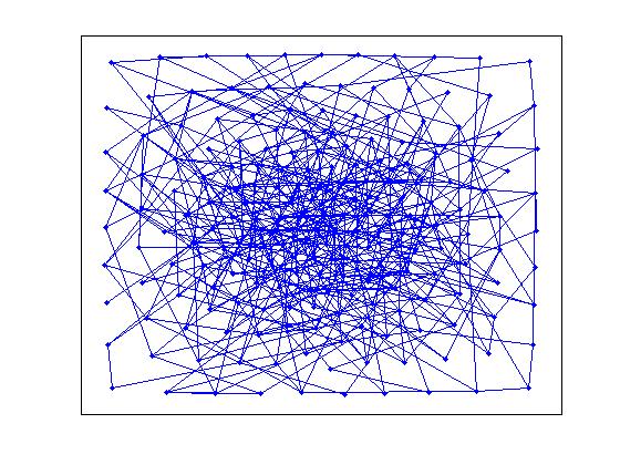
Using the Matlab interface to the AT&T Graphvis program neato, we can generate a layout
for this graph and visualize it using the matlab gplot function. That way, we can see if
it really does have a giant component.
>> [x y] = draw_dot(G);
>> gplot(G, [x' y'], '.-');
In the center of the picture, we see the large connected component of the graph.
Evolution
Now that we know how to generate Erdos-Reyni random graphs,
let's look at how they evolve in p -- the probability of an edge between two nodes.
Effectively, as we keep adding edges randomly to a graph, what happens?
From theory, we expect to see a giant component with approximately log(n) vertices
emerge when p is near 1/(n-1). Then, we expect the graph to become completely connected
when p is close to log(n)/n.
First, we need to setup our graph as a function of p. The new anonymous functions
in Matlab 7 make this easy.
>> n = 200;
>> A = rand(n,n);
>> A = triu(A,1);
>> A = A + A';
>> G = @(p) A < p;
Now, let's compute the thresholds and look at the graph near the thresholds.
>> thres_conn = log(n)/n
thres_conn =
0.0265
>> thres_giant = 1/(n-1)
thres_giant =
0.0050
For each graph, we generate coordinates using the AT&T Graphvis tool, and then plot using Matlab's gplot.
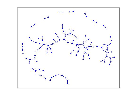
>> [x y] = draw_dot(G(thres_giant));
>> gplot(G(thres_giant), [x' y'], '.-')
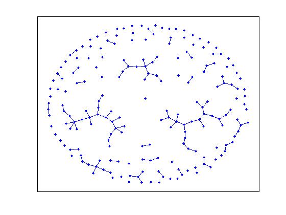
>> [x y] = draw_dot(G(thres_conn));
>> gplot(G(thres_conn), [x' y'], '.-')
While the second picture is definitely connected, the former doesn't appear to have a giant
component. Remember that we aren't guaranteed to find a giant component at this p, but it has
to happen soon. In this case, notice that it is very likely that the two larger components
will merge together very soon.
Now, let's animate the result. To do this, let's generate a layout at the geometric mean
of the connected threshold and the giant component threshold. (I'm not sure why
that probability is a good one to use for drawing the graph, but it happens to work
well in practice.)
>> [x y] = draw_dot(G(sqrt(thres_conn*thres_giant)));
The following script animation script depends on the largest_component
function which is not standard to Matlab and uses the components function
from the meshpart toolkit.
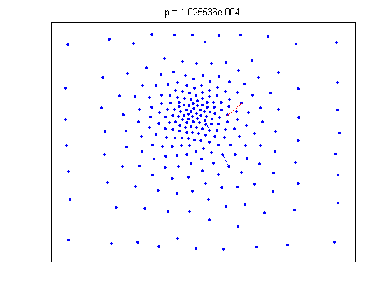
t1 = linspace(0, thres_giant, 50);
t2 = linspace(thres_giant, thres_conn, 100);
t = [t1 ones(1,40)*thres_giant t2];
for (tt = t)
% plot the graph
gplot(G(tt), [x' y'], 'b.-');
hold on;
% plot the largest component of the graph
[Glc p] = largest_component(G(tt));
gplot(Glc, [x(p)' y(p)'], 'r');
hold off;
set(gca, 'YTick', []);
set(gca, 'XTick', []);
set(gcf, 'Color', [1 1 1]);
title(sprintf('p = %d', tt));
pause(0.15);
end;

The animation pauses briefly at the component where a giant threshold emerges.
I've provided three more examples of these plots for