Evolution of the giant connected component

In the last example, we saw how an Erdos-Renyi graph has a giant connected component when the connection probability exceeds a threshold. In this script, we will watch the evolution process closely. This script is designed to be run locally, because it produces an animated figure with many subplots. The HTML fill will produce a few presentative examples.

Contents

Parameterize the Erdos-Renyi graph

Here, we first create a parametric representation of varying the connection probability in an Erdos-Renyi random graph.

rand('seed',100);
n = 150;
A = rand(n);
A = triu(A,1);
A = A + A'; % make sure the seed data is symmetric

% define a function to produce a graph given a probability
G = @(p) A < p;

Define thresholds for the Erdos-Renyi graph

% define the thresholds where the graph is fully connected and has
% a giant component
thres_conn = log(n)/(n);
thres_giant = 1/(n-1);

% define a layout threshold at the geometric mean of these thresholds
thres = sqrt(thres_conn*thres_giant);

Compute a static layout

find the layout at the given threshold

Gt = G(thres);
[x y] = neato_layout(Gt);

Show the graph's evolution

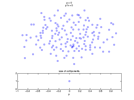
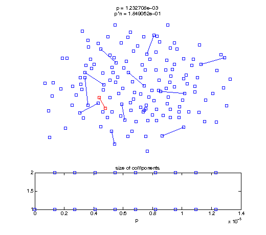
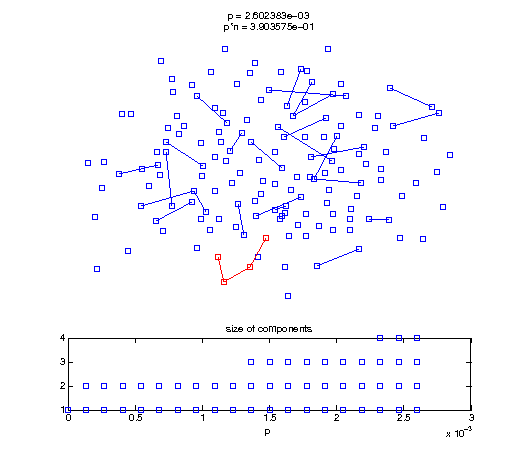
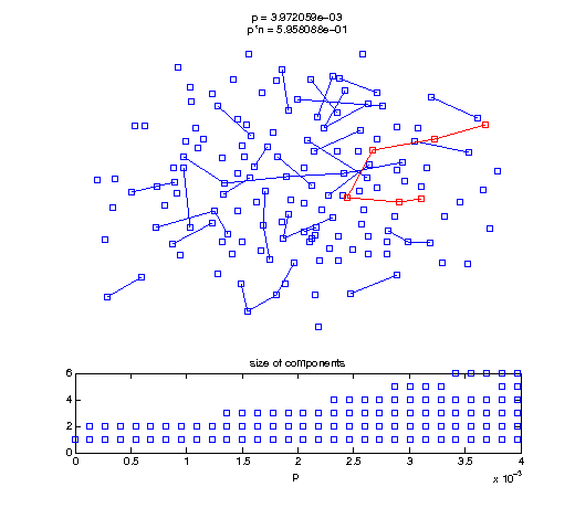
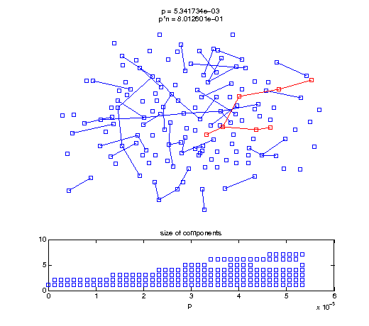
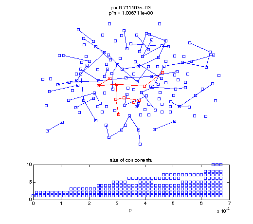
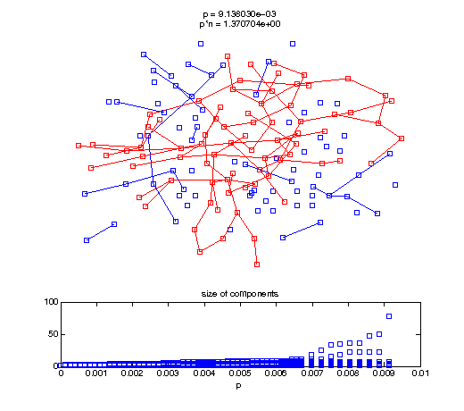
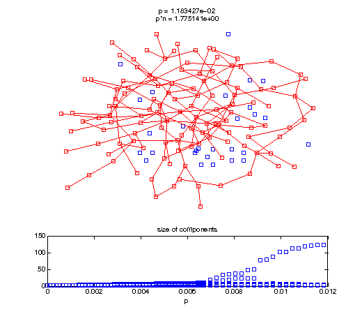
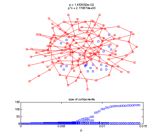
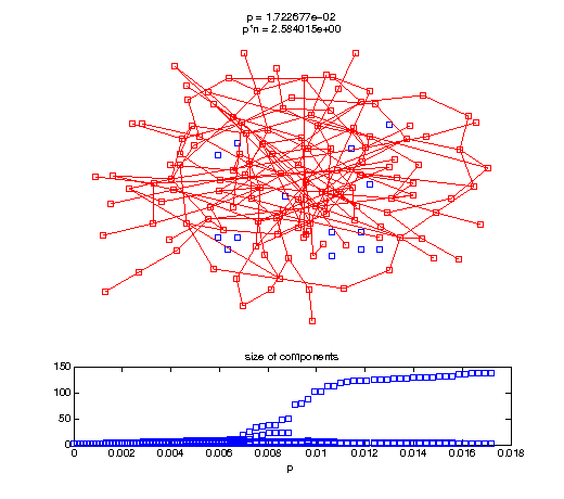
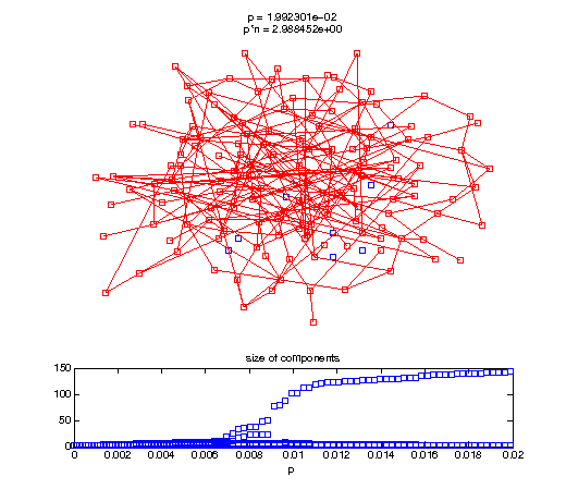
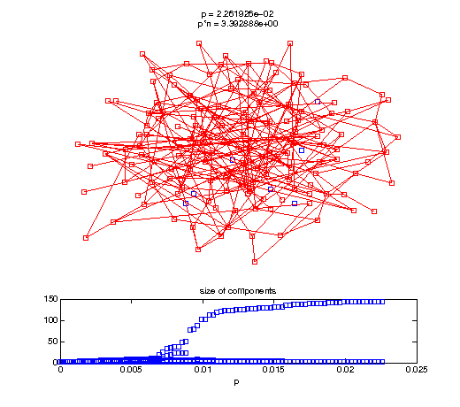
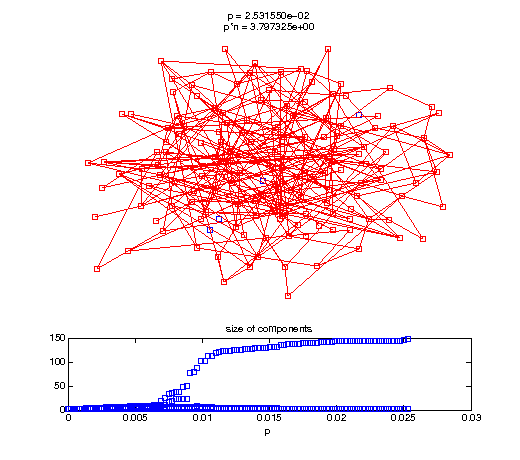
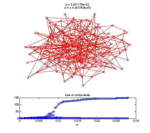
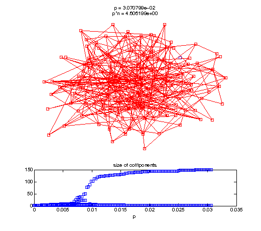
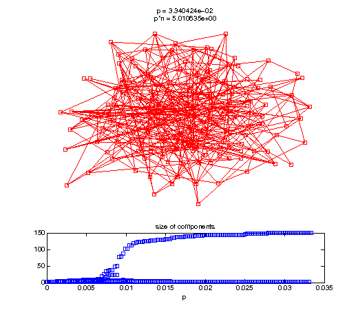
Now, we'll watch as the graph evolves as we keep adding edges by increasing the probability p through all the various thresholds.

Define a sequence of probabilities to explore.

t1 = linspace(0, thres_giant, 50);
t2 = linspace(thres_giant, thres_conn, 100);

% we want to pause things at the emergence of the giant component
steps = [t1 ones(1,40)*thres_giant t2];
nframes = length(steps);

comp_size_history = [];
comp_step_history = [];

for frame=1:nframes
    p = steps(frame);

    Gcur = G(p);

    % make one large subplot for the graph layout with the
    % giant component highlighted
    subplot(4,2,[1 2 3 4 5 6]);
    gplot(Gcur, [x' y'],'bo-'); hold on;
    plot(x', y', 'bo');
    [Glc pcc] = largest_component(Gcur);
    gplot(Glc, [x(pcc)' y(pcc)'], 'ro-');
    hold off;
    axis off;
    title({sprintf('p = %d', p), sprintf('p*n = %d', p*n)});

    % make a smaller subplot for the size of the components
    subplot(4,2,[7 8]);
    [comps comp_sizes] = components(Gcur); % get the sizes
    comp_size_history = [comp_size_history comp_sizes];
    comp_step_history = [comp_step_history ones(1,length(comp_sizes))*p];
    plot(comp_step_history, comp_size_history, 'o');
    title('size of components');
    xlabel('p');

    set(gcf,'Color',[1,1,1]);

    % pause for display
    pause(0.15);
    if mod(frame,10)==0 || frame==1 || frame==nframes, snapnow; end
end

Published with MATLAB® 7.12