This text is adapted from Numerical Methods by Greenbaum and Chartier and is meant as a Julia-based analogue to their chapter on Matlab.
Julia is a high-level programming language that can be used for any technical or numerical computing problem, but is especially well-suited to linear algebra computations. It is also a powerful general-purpose programming language in its own right.
In this course, we think that juliabox.com is the best way to run Julia. This uses the jupyter notebook interface that enables us to insert commands and see their results.
To use this, enter juliabox.com in your browser.
(Note, there is an older juliabox.org website that serves the same purpose, but please use juliabox.com for CS314 at Purdue in Fall 2016.)
You should see the following webpage.

At this point, you need to login to juliabox. I do it via Google, which uses your google id, but has no other access to your account.
Once you do that, you'll get to the file browser.

This allows you to create new notebooks (the New button at the upper-right...) or work through a directory structure. All the files are stored on Google's cloud and saved so that they'll be there if you return. You can upload files through the "Files" button at top.
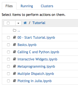
The Tutorial is placed by default in every new juliabox setup. (Only once though, if you delete it, I don't know how to get it back right now.) This is a good place to start. If you click on the tutorial, you'll get a list of notebooks.

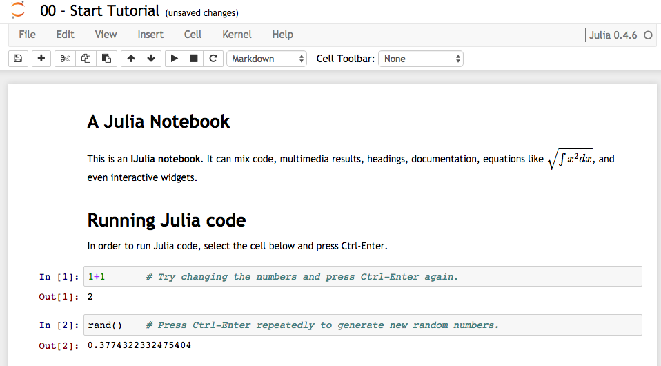
Once you click on a notebook (say the 00 - Start Tutorial.ipnb file), then you'll start a notebook!

Actually, this file is a notebook itself, so we can type commands just the same way!
These examples now follow your textbook. To create a new "cell", go to "Insert Cell Below" and you'll get your own area to type commands
1+2*3
ans/4
Section 2.2 - Vectors
At this point, we are going to switch back and show how to do the commands in the book
v = [1; 2; 3; 4]
v = [1.; 2; 3; 4]
w = [5 6 7 8]
w = map(Float64,[5 6 7 8]) # convert to Float64
v[2]
w[3]
v+w
v+w'
vec(v+w')
v[1]+v[2]+v[3]+v[4]
sumv = 0.
for i=1:4
    sumv = sumv+v[i];
end
sumv
(Section 2.3) Getting help
?sum
David's note. Julia's documentation is currently not as good as Matlab's :(
Section 2.4 Matrices
A = [1 2 3; 4 5 6; 7 8 0]
b = [0; 1; 2]
x = A\b
Show a full precision answer. This is slightly easier in Matlab.
for i=1:length(x)
    @printf("%.16e\n", x[i])
end
x
b - A*x
Section 2.6 Comments
#Section 2.6 Comments
#Solve Ax = b
x = A\b # this solves Ax=b and stores the result for x
Warning
We are still editing the section below this!
#2.8 Creating your own functions
f(x) = x^2 + 2x
f(5)
map(f, 0:1:5)
x -> x^2 + 2x #Anonymous function
map(x -> x^2 + 2x, 0:1:5)
#2.9 Printing
x = 0:.5:2
print(x)
@printf("x = %s" ,collect(x))
y = rand(5,3)
println("      Score1            Score2             Score3 ")
println("$y")
println("      x \t\t sqrt(x) \n=====================================")
for x=1:5
    @printf("%f \t\t %f\n",x, sqrt(x))   #formating string
end
#2.10 More Loops and Conditionals
using Plots
print("Enter initial xmin ")
xmin = parse(Float64, readline())
print("Enter initial xmax ")
xmax = parse(Float64, readline())
print("Enter tolerance ")
tolerance = parse(Float64, readline())

while xmax - xmin > tolerance
  x = collect(xmin:(xmax-xmin)/100:xmax)
  y = map(x->x^2, x)
  plot!(x,y)
  print("Enter new value for xmin ")
  xmin = parse(Float64, readline())
  print("Enter new value for xmax ")
  xmax = parse(Float64, readline())
end